Site pages
Current course
Participants
General
Module 1. Average and effective value of sinusoida...
Module 2. Independent and dependent sources, loop ...
Module 3. Node voltage and node equations (Nodal v...
Module 4. Network theorems Thevenin’ s, Norton’ s,...
Module 5. Reciprocity and Maximum power transfer
Module 6. Star- Delta conversion solution of DC ci...
Module 7. Sinusoidal steady state response of circ...
Module 8. Instantaneous and average power, power f...
Module 9. Concept and analysis of balanced polypha...
Module 10. Laplace transform method of finding ste...
Module 11. Series and parallel resonance
Module 12. Classification of filters
Module 13. Constant-k, m-derived, terminating half...
LESSON 31. m-derived filters
31.1 m-Derived T-Section
It is clear from previous chapter Figs 30.3 & 30.7 that the attenuation is not sharp in the stop band for k-type filters. The characteristic impedance, Z0 is a function of frequency and varies widely in the transmission band. Attenuation can be increased in the stop band by using ladder section, i.e. by connecting two or more identical sections. In order to join the filter sections, it would be necessary that their characteristic impedance be equal to each other at all frequencies. If their characteristic impedances match at all frequencies, they would also have the same pass band. However, cascading is not a proper solution from a practical point of view. This is because practical elements have a certain resistance, which gives rise to attenuation in the pass band also. Therefore, any attempt to increase attenuation in stop band by cascading also results in an increase of ‘a’ in the pass band. If the constant k section is regarded as the prototype, it is possible to design a filter to have rapid attenuation in the stop band, and the same characteristic impedance as the prototype at all frequencies. Such a filter is called m-derived filter. Suppose a prototype T-network shown in Fig.31.1 (a) has the series arm modified as shown in Fig.31.1 (b), where m is a constant. Equating the characteristic impedance of the networks in Fig.31.1, we have
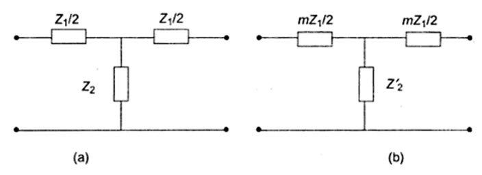
Fig.31.1
Z0T = Z0T’
where Z0T’ is the characteristic impedance of the modified (m-derived) T-network
\[\sqrt {{{Z_1^2} \over 4} + {Z_1}{Z_2}}=\sqrt {{{{m^2}Z_1^2} \over 4} + m{Z_1}Z_2^1}\]
\[{{Z_1^2} \over 4} + {Z_1}{Z_2}={{{m^2}Z_1^2} \over 4} + m{Z_1}Z_2^1\]
\[m{Z_1}Z_2^1={{Z_1^2} \over 4}\left( {1 - {m^2}} \right) + {Z_1}{Z_2}\]
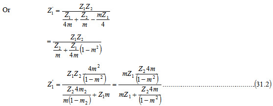
\[Z_2^1={{{Z_1}} \over {4m}}\left( {1 - {m^2}} \right) + {{{Z_2}} \over m}...................................................\left( {31.1} \right)\]
It appears that the shunt arm \[Z_2^1\] consider of two impedance in series as shown in Fig.31.2
From Eq.31.1, \[{{1 - {m^2}} \over {4m}}\] should be positive to realize the impedance \[Z_2^1\] physically, i.e. 0<m<1. Thus m-derived section can be obtained from the prototype by modifying its series and shunt arms. The same technique can be applied to \[\pi\] section network. Suppose a prototype p-network shown in Fig.31.3 (a) has the shunt arm modified as shown in Fig.31.3 (b).
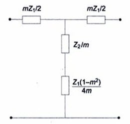
Fig.31.2
The characteristic impedances of the prototype and its modified sections have to be equal for matching.
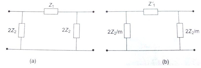
Fig.31.3
\[Z0\pi=Z_{0\pi }^1\]
where \[Z_{0\pi }^1\] is the characteristic impedance of the modified (m-derived) \[\pi\]-network.
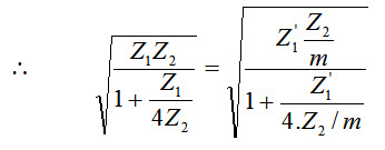
Squaring and cross multiplying the above equation results as under.
\[\left( {4{Z_1}{Z_2} + mZ_1^'{Z_1}} \right)={{4Z_1^'{Z_2} + {Z_1}Z_1^'} \over m}\]
\[Z_1^'\left( {{{{Z_1}} \over m} + {{4{Z_2}} \over m} - m{Z_1}} \right)=4{Z_1}{Z_2}\]
It appears that the series arm of the m-derived \[\pi\] section is a parallel combination of mZ1 and 4mZ2/1-m2. The derived m section is shown in Fig.31.4
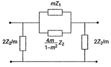
Fig.31.4
m-Derived Low Pass Filter
In Fig.31.5, both m-derived low pass T and \[\pi\] filter sections are shown. For the T-section shown Fig.31.5 (a), the shunt arm is to be chosen so that it is resonant at some frequency ƒx above cut-off frequency ƒc its impedance will be minimum or zero. Therefore, the output is zero and will correspond to infinite attenuation at this particular frequency. Thus, at ƒx.
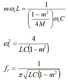
\[{1 \over {m{\omega _r}C}}={{1 - {m^2}} \over {4m}}{\omega _r}L,\] where ω, is the resonant frequency
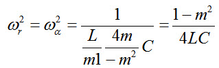
\[{{1 - {m^2}} \over {4m}}C\]
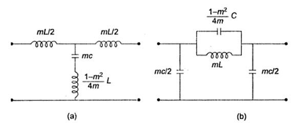
Fig.31.5
\[\omega _r^2={4 \over {\left( {1 - {m^2}} \right)LC}}\]
\[{f_r}={1 \over {\pi \sqrt {LC\left( {1 - {m^2}} \right)} }}={f_x}\]
Since the cut-off frequency for the low pass filter is \[{f_c}={1 \over {\pi \sqrt {LC} }}\]
\[{f_x}={{{f_c}} \over {\sqrt {1 - {m^2}} }}...................................................\left( {31.3} \right)\]
or \[m=\sqrt {1 - {{\left( {{{{f_c}} \over {{f_\alpha }}}} \right)}^2}} ...................................................\left( {31.4} \right)\]
If a sharp cut-off is desired, ƒx should be near to ƒc, From Eq.31.3, it is clear that for the smaller the value of m, ƒ\[\propto\] comes close to ƒc, . Equation 31.4 shows that if ƒc and ƒ\[\propto\] are specified, the necessary value of m may then be calculated. Similarly, for m –derived \[\pi\] section, the inductance and capacitance in the series arm constitute a resonant circuit. Thus, at ƒx a frequency corresponds to infinite attenuation, i.e. at ƒx.
Since, \[{f_c}={1 \over {\pi \sqrt {LC} }}\]
\[{f_r}={{{f_c}} \over {\sqrt {1 - {m^2}} }}={f_\alpha }...................................................\left( {31.5} \right)\]
Thus for both m-derived low pass networks for a positive value of m (0< m <1), ƒx > ƒc. Equations 31.4 or 31.5 can be used to choose the value of m, knowing ƒc and ƒr. After the value of m is evaluated, the elements of the T or p-network can be found from Fig.31.5. The variation of attenuation for a low pass m-derived section can be verified from \[\alpha\] = 2 cosh-1 \[\sqrt {{Z_1}/4{Z_2}} \,for\,{f_c} < f < {f_\alpha }.\] For Z1 = jωL and Z1 =-J/ωC for the prototype.
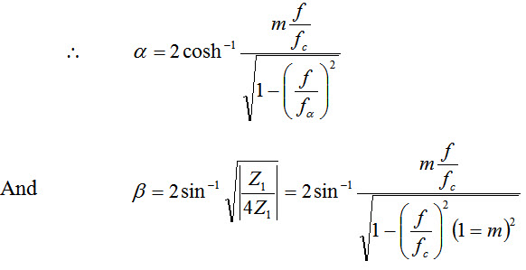
Figure 31.6 shows the variation of \[\alpha\] , β and Z0 with respect to frequency for an m-derived low pas filter.
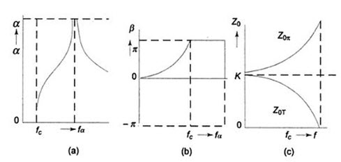
Fig.31.6
m-derived High Pass Filter
In Fig.31.7 both m-derived high pass T and \[\pi\]-sections are shown.
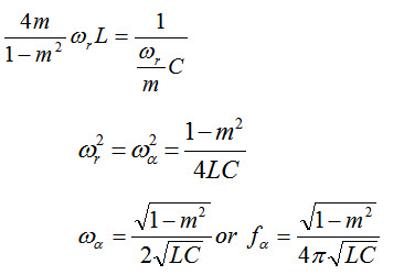
If the shunt arm in T-section is series resonant, it offers minimum or zero impedance. Therefore, the output is zero and, thus, at resonance frequency, or the frequency corresponds to infinite attenuation.
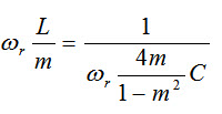
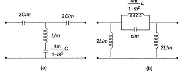
Fig.31.7
\[{\omega _\alpha }={{\sqrt {1 - {m^2}} } \over {2\sqrt {LC} }}or\,\,{f_\alpha }={{\sqrt {1 - {m^2}} } \over {4\pi \sqrt {LC} }}\]
From Eq.30.6, the cut-off frequency fc of a high pass prototype filter is given by
\[{f_c}={1 \over {4\pi \sqrt {LC} }}\]
\[{f_\alpha }={f_c}\sqrt {1 - {m^2}} ...................................................\left( {31.6} \right)\]
\[m=\sqrt {1 - {{\left( {{{{f_\alpha }} \over {{f_c}}}} \right)}^2}} ...................................................\left( {31.7} \right)\]
Similarly, for the m-derived \[\pi\]-section, the resonant circuit is constituted by the series arm inductance nd capacitance. Thus, at ƒx.
Thus, the frequency corresponding to infinite attenuation is the same for both sections.
Equation 31.7 may be used to determine m for a given ƒx and ƒc. The elements of the m-derived high pass T or \[\pi\]-sections can be found from Fig.31.7. The variation of \[\alpha\], β and Z0 with frequency is shown in Fig.31.8
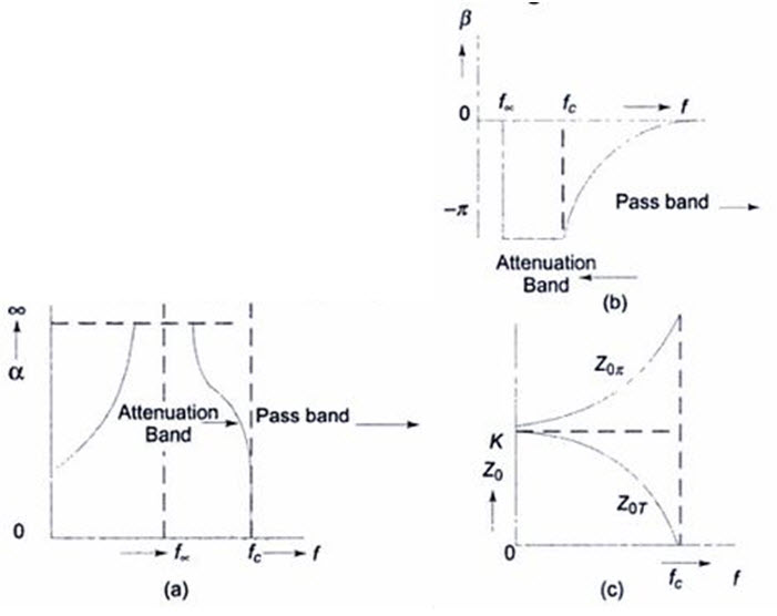
Fig. 31.8
Last modified: Monday, 30 September 2013, 9:11 AM