Electrical Circuits 3(2+1)

LESSON 32. Terminating half network and composite filters

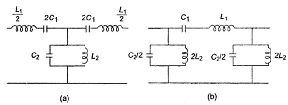Fig.32.1

For this condition of equal resonant frequencies.

                       \[{\omega _0}{{{L_1}} \over 2}={1 \over {2{\omega _0}{C_1}}}\,\,for\,\,the\,\,sereis\,\,arm\]

From which,  \[\omega _0^2{L_1}{C_1}=1...................................................\left( {32.1} \right)\]

and      \[{1 \over {{\omega _0}{C_2}}}={\omega _0}{L_2}\,for\,the\,shunt\,arm\]

from which,   \[\omega _0^2{L_2}{C_2}=1...................................................\left( {32.2} \right)\]

          \[\omega _0^2{L_1}{C_1}=1=\omega _0^2{L_2}{C_2}\]

\[{L_1}{C_1}={L_2}{C_2}...................................................\left( {32.3} \right)\]

The impedance of the series arm, Z₁ is given by

          \[{Z_1}=\left( {j\omega {L_1} - {j \over {\omega {C_1}}}} \right)=j\left( {{{{\omega ^2}{L_1}{C_1} - 1} \over {\omega {C_1}}}} \right)\]

The impedance of the shunt arm, Z₂ is given by

                       

\[{Z_1}{Z_2}=j\left( {{{{\omega ^2}{L_1}{C_1} - 1} \over {\omega {C_1}}}} \right)\left( {{{j\omega {L_2}} \over {1 - {\omega ^2}{L_2}{C_2}}}} \right)\]

                      \[={{ - {L_2}} \over {{C_1}}}\left( {{{{\omega ^2}{L_1}{C_1} - 1} \over {1 - {\omega ^2}{L_2}{C_2}}}} \right)\]

From Eq.32.3, L₁C₁ = L₂C₂

                      \[{Z_1}{Z_2}={{{L_2}} \over {{C_1}}}={{{L_1}} \over {{C_2}}}={k^2}\]

Where k is constant. Thus, the filter is a constant k-type. Therefore, for a constant k-type in the pass band.

                       \[- 1 < {{{Z_1}} \over {4{Z_2}}} < 0,\,\,and\,\,at\,cut - off\,frequency\]

                        Z₁ = 4Z₂

                       \[Z_1^2=-4{Z_1}{Z_2}=-4{k^2}\]

\[{Z_1}=\pm j2k\]

i.e. the value of Z₁ at lower cut-off frequency is equal to the negative of the value of Z₁ at the upper cut-off frequency.

\[\left( {{1 \over {j{\omega _1}{C_1}}} + j{\omega _1}{L_1}} \right)=-\left( {{1 \over {j{\omega _2}{C_1}}} + j{\omega _2}{L_1}} \right)\]

or           \[\left( {{\omega _1}{L_1}{1 \over {{\omega _1}{C_1}}}} \right)=\left( {{1 \over {{\omega _2}{C_1}}} - {\omega _2}{L_1}} \right)\]

\[\left( {1 - \omega _1^2{L_1}{C_1}} \right)={{{\omega _1}} \over {{\omega _2}}}\left( {\omega _2^2{L_1}{C_1} - 1} \right)...................................................\left( {32.4} \right)\]

From Eq.32.1, \[{L_1}{C_1}={1 \over {\omega _0^2}}\]

Hence Eq.32.4 may be written as

\[\left( {1 - {{\omega _1^2} \over {\omega _0^2}}} \right)={{{\omega _1}} \over {{\omega _2}}}\left( {{{\omega _2^2} \over {\omega _0^2}} - 1} \right)\]

\[\left( {\omega _0^2 - \omega _1^2} \right){\omega _2}={\omega _1}\left( {\omega _2^2 - \omega _0^2} \right)\]

\[\omega _0^2{\omega _2} - \omega _1^2{\omega _2}={\omega _1}\omega _2^2 - {\omega _1}\omega _0^2\]

\[\omega _0^2\left( {\omega _1^{} + {\omega _2}} \right)={\omega _1}{\omega _2}\left( {{\omega _2} + {\omega _1}} \right)\]

\[\omega _0^2={\omega _1}{\omega _2}\]

\[{f_0}=\sqrt {{f_1}{f_2}} ...................................................\left( {32.5} \right)\]

\[{Z_1}=-2jk\]

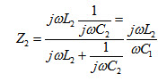
Thus, the resonant frequency is the geometric mean of the cut-off frequencies.  The variation of the reactances with respect to frequency is shown in Fig.32.2

Design. If the filter is terminated in a load resistance R=K, then at the lower cut-off frequency.

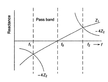
Fig.32.2

\[\left( {{1 \over {j{\omega _1}{C_1}}} + j{\omega _1}{L_1}} \right)=-2jk\]

\[{1 \over {{\omega _1}{C_1}}}-{\omega _1}{L_1}=2k\]

        \[1 - \omega _1^2{C_1}{L_1} - 2k{\omega _1}{C_1}\]

Since    \[{L_1}{C_1}={1 \over {\omega _0^2}}\]

              \[1 - {{\omega _1^2} \over {\omega _0^2}}=2k{\omega _1}{C_1}\]

or          \[1 - {\left( {{{{f_1}} \over {{f_0}}}} \right)^2}=4\pi k{f_1}{C_1}\]

              \[1 - {{f_1^2} \over {{f_1}{f_2}}}=4\pi k{f_1}{C_1} & \left( {{f_0}=\sqrt {{f_1}{f_2}} } \right)\]

              \[{f_2} - {f_1}=4\pi k{f_1}{f_2}{C_1}\]

               \[{C_1}={{{f_2} - {f_1}} \over {4\pi k{f_1}{f_2}}}...................................................\left( {32.6} \right)\]

Since      \[{L_1}{C_1}={1 \over {\omega _0^2}}\]

                       \[{L_1}={1 \over {\omega _0^2{C_1}}}={{4\pi k{f_1}{f_2}} \over {\omega _0^2\left( {{f_2} - {f_1}} \right)}}\]

                       \[{L_1}={k \over {\pi \left( {{f_2} - {f_1}} \right)}}...................................................\left( {32.7} \right)\]

To evaluate the values for the shunt arm, consider the equation

                       \[{Z_1}{Z_2}={{{L_2}} \over {{C_1}}}={{{L_1}} \over {{C_2}}}={k^2}\]

\[{L_2} = {C_1}{k_2}={{\left( {{f_2} - {f_1}} \right)k} \over {4\pi {f_1}{f_2}}}...................................................\left( {32.8} \right)\]

and          \[{C_2}={{{L_1}} \over {{k^2}}}={1 \over {\pi \left( {{f_2} - {f_1}} \right)k}}...................................................\left( {32.9} \right)\]

Equations 32.6 through 32.9 are the design equations of a prototype band pass filter.  The variation of a, b with respect to frequency is shown in Fig.32.3.

Fig.32.3

32.2. Band Elimination Filter

A band elimination filter is one which passes without attenuation all frequencies less than the lower cut-of frequency ƒ_z, and greater than the upper cut-off frequency ƒ₂. Frequencies lying between ƒ₁ and ƒ₂ are attenuated.  It is also known as band stop filter.  Therefore, a band stop filter can be realized b connecting a low pass filter in parallel with a high pass section, in which the cut-off frequency of low pass filter is below that of a high pass filter.  The configurations of T and \[\pi\] constant k band to sections are shown in Fig.32.4.  The band elimination filter is designed in the same manner as is the band pass filter.

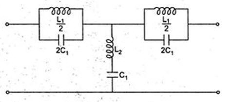
Fig.32.4

As for the band pass filter, the series and shunt arms are chosen to resonate at the same frequency ω₀.  Therefore, from Fig.32.1 (a), for the condition of equal resonant frequencies.

                       \[{{{\omega _0}{L_1}} \over 2}={1 \over {2{\omega _0}{C_1}}}\,\,for\,\,the\,\,series\,\,arm\]

or            \[\omega _0^2={1 \over {{L_1}{C_1}}}...................................................\left( {32.10} \right)\]

\[{\omega _0}{L_2}={1 \over {{\omega _0}{C_2}}}\,\,for\,\,the\,\,shunt\,\,arm\]

                      \[\omega _0^2={1 \over {{L_2}{C_2}}}...................................................\left( {32.11} \right)\]

                       \[{1 \over {{L_1}{C_1}}}={1 \over {{L_2}{C_2}}}=k\]

Thus                L₁C₁ = L₂C₂

            It can be also verified that

                     \[{Z_1}{Z_2}={{{L_1}} \over {{C_2}}}={{{L_2}} \over {{C_1}}} = {k^2}...................................................\left( {32.13} \right)\]

and        \[{f_0}=\sqrt {{f_1}{f_2}} ...................................................\left( {32.14} \right)\]

At cut-off frequencies, Z₁ = -4Z₂

Multiplying both sides with Z₂, we get

             \[{Z_1}{Z_2}=-4Z_2^2={k^2}\]

       \[{Z_2}=\pm j{k \over 2}...................................................\left( {32.15} \right)\]

If the load is terminated in a load resistance, R = k, then at lower cut-off frequency

              \[{Z_2}=j\left( {{1 \over {{\omega _1}{C_2}}} - {\omega _1}{L_2}} \right)=j{k \over 2}\]

               \[{1 \over {{\omega _1}{C_2}}} - {\omega _1}{L_2}={k \over 2}\]

                \[1 - \omega _1^2{C_2}{L_2}={\omega _1}{C_2}{k \over 2}\]

From Eq. 32.11, \[{L_2}{C_2}={1 \over {\omega _0^2}}\]

                       \[1 - {{\omega _1^2} \over {\omega _0^2}}={k \over 2}{\omega _1}{C_2}\]

                       \[1 - {\left( {{{{f_1}} \over {{f_0}}}} \right)^2}=k\pi {f_1}{C_2}\]

                       \[{C_2}={1 \over {k\pi {f_1}}}\left[ {1 - {{\left( {{{{f_1}} \over {{f_0}}}} \right)}^2}} \right]\]

since       \[{f_0}=\sqrt {{f_1}{f_2}}\]

                \[{C_2}={1 \over {k\pi }}\left[ {{1 \over {{f_1}}} - {1 \over {{f_2}}}} \right]\]

                 \[{C_2}={1 \over {k\pi }}\left[ {{{{f_2} - {f_1}} \over {{f_1}{f_2}}}} \right]...................................................\left( {32.16} \right)\]

From Eq.32.11, \[\omega _0^2={1 \over {{L_2}{C_2}}}\]

                  \[{L_2}={1 \over {\omega _0^2{C_2}}}={{\pi k{f_1}{f_2}} \over {\omega _0^2\left( {{f_2} - {f_1}} \right)}}\]

Since         \[{f_0}=\sqrt {{f_1}{f_2}}\]

                  \[{L_2}={k \over {4\pi \left( {{f_2} - {f_1}} \right)}}...................................................\left( {32.17} \right)\]

Also from Eq.32.13,

                       \[{k^2}={{{L_1}} \over {{C_2}}}={{{L_2}} \over {{C_1}}}\]

                       \[{L_1}={k^2}{C_2}={k \over \pi }\left( {{{{f_2} - {f_1}} \over {{f_1}{f_2}}}} \right)...................................................\left( {32.18} \right)\]

and        \[{C_1}={{{L_2}} \over {{k^2}}}...................................................\left( {32.19} \right)\]

                     \[={1 \over {4\pi k\left( {{f_2} - {f_1}} \right)}}\]

The variation of the reactances with respect to frequency is shown in Fig.32.5

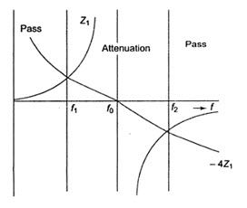
Fig.32.5

Equation 32.16 through Eq.32.19 are the design equations of a prototype band elimination filter.  The variation of \[\alpha\], β with respect to frequency is shown in Fig.32.6

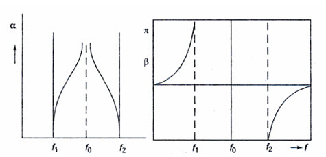
Fig.32.6

32.3 Composite filter

A composite filter is an electronic filter consisting of multiple filter sections of two or more different types.

The method of filter design determines the properties of filter sections by calculating the properties they have in an infinite chain of such sections. In this, the analysis parallels transmission line theory on which it is based. Filters designed by this method are called  parameter filters, or just  filters. An important parameter of filters is their impedance, the impedance of an infinite chain of identical sections.

The basic sections are arranged into a ladder network of several sections, the number of sections required is mostly determined by the amount of stop band rejection required. In its simplest form, the filter can consist entirely of identical sections. However, it is more usual to use a composite filter of two or three different types of section to improve different parameters best addressed by a particular type. The most frequent parameters considered are stop band rejection, steepness of the filter skirt (transition band) and impedance matching to the filter terminations.  Filters are linear filters and are invariably also passive in implementation.