Ground Water, Wells and Pumps

Lesson 10 Steady Groundwater Flow to Wells

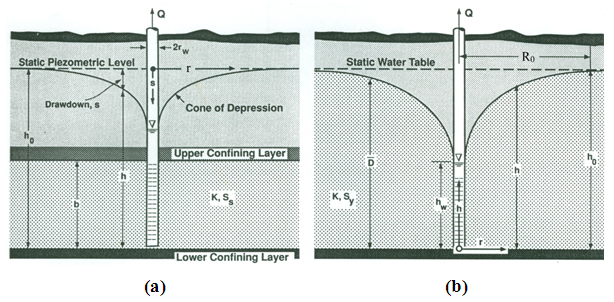
Fig. 10.1. Drawdown pattern in: (a) Confined aquifer; (b) Unconfined aquifer. (Source: Roscoe Moss Company, 1990)

 

The difference between the static water level and the pumping water level at any instant is called ‘drawdown’, which is a function of pumping rate, pumping duration and distance from the pumping well. Drawdown is always maximum at the pumping well and it decreases with an increase in the distance from pumping well (Fig. 10.1). The rate of pumping from an aquifer significantly affects the hydraulic gradient in the aquifer. The faster the well is pumped, the steeper the hydraulic gradient will be in the vicinity of the well.  

 

A drawdown curve at a given time shows the variation of drawdown with distance from the pumping well. In three dimensions, the drawdown curve takes the shape of an inverted cone centered on the pumping well, which is known as cone of depression. The outer limit of the cone of depression defines the area of influence of the well. The boundary of the area of influence is called circle of influence and the radius of the circle of influence is called radius of influence. Thus, the radius of influence (R₀) is the distance from a pumping well to the edge of the cone of depression (Fig. 10.1) where drawdown is zero.

 

As more and more groundwater is pumped through the well, the more water comes from aquifer storage. As a result, the radius of influence increases until when the rate of pumping (discharge) becomes equal to the rate of flow into the well from the area around the well. At this instant of time, a steady flow condition exists in the aquifer and the cone of depression gets stabilized (i.e., it does not change with pumping time). This equilibrium condition changes when the pumping rate is increased or decreased. Note that under steady-state conditions, the entire pumped water is assumed to be coming from external sources beyond the radius of influence. In contrast, under unsteady-state (transient-flow) conditions, either entire pumped water is assumed to be coming from the aquifer storage within the radius of influence or the pumped water is assumed to be coming partly from the aquifer storage within the radius of influence and partly from external sources beyond the radius of influence depending on field conditions.        

 

In this lesson, the main equations for analyzing steady flow to fully penetrating wells in confined and unconfined aquifers are derived and their applications are discussed. In addition, the concept of partial penetration and the equations for computing steady drawdown in partially penetrating wells installed in confined and unconfined aquifers are presented.  

     

10.2 Steady Flow to Fully Penetrating Wells

10.2.1 Basic Assumptions for Analyzing Flow to Wells

The following are the basic assumptions made for analyzing flow to wells:

1. The aquifer is bounded on the bottom by a confining layer.
2. The groundwater level of the aquifer is horizontal and not changing with time prior to the start of pumping.
3. All changes in the position of the groundwater level are due to the effect of the pumping well alone.
4. All geologic formations are horizontal and of infinite horizontal extent.
5. The aquifer is homogeneous and isotropic.
6. All flow is radial towards the well.
7. Groundwater flow is horizontal.
8. Darcy’s law is valid.
9. The pumping well and the observation wells are fully penetrating.
10. The pumping well has an infinitesimal diameter (i.e., negligible storage) and is 100% efficient (i.e., no well losses).
11. Groundwater has a constant density and viscosity.

 

10.2.2 Radial Symmetry

The flow towards a well is termed radial flow. Radial flow can be thought of as flow along the spokes of a wagon wheel towards the hub. Besides the above-mentioned basic assumptions, it is also assumed that flow to wells is radially symmetric. This means that the values of aquifer transmissivity (T) and storage coefficient (S) do not depend on the direction of flow in the aquifer. Although solutions can be found for cases in which the value of the horizontal hydraulic conductivity is different from that of the vertical hydraulic conductivity, it usually assumed that the aquifer has radial symmetry.

 

10.2.3 Steady-State Condition

As mentioned above, if pumping is continued for a long time, the groundwater level may reach a state of equilibrium, i.e., no change in drawdown with time. When the equilibrium (steady-state) condition is achieved, the cone of depression stops growing because it reaches a recharge boundary which contributes all flow to the well. The hydraulic gradient of the cone of depression causes water to flow at a constant rate from the recharge boundary to the well. Such a hydraulic condition in the aquifer is known as a steady flow condition. The assumption of radial symmetry means that the recharge boundary has an unlikely circular geometry entered about the pumping well! In this lesson, our focus is to analyze the steady flow to pumping wells, and hence it is also assumed that flow towards the well is under steady-state conditions.   

 

10.2.4 Steady Radial Flow in Confined Aquifers

For analyzing steady radial flow in a confined aquifer, apart from the above assumptions, the following additional assumptions are necessary:

• The aquifer is bounded on the top and bottom by impervious confining layers (i.e., there is no leakage through confining layers).
• The well is pumped at a constant rate.

 

Figure 10.2 shows a pumping well fully penetrating a confined aquifer and is subjected to pumping. Groundwater level under equilibrium conditions is also depicted. Under equilibrium (steady-state) conditions, the rate of pumping (Q) is equal to the rate that the aquifer transmits water to the well. This problem was first solved by G. Thiem in 1906, which is presented below. 

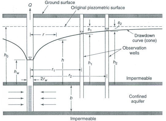
Fig. 10.2. Steady flow to a pumping well in a confined aquifer.

(Source: Todd, 1980)

 

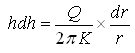
From the Darcy’s law, the flow of water through a circular section of the aquifer towards the pumping well is given as:

 

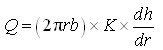                                                                                 (10.1)

 

Where, Q = constant rate of pumping from the well, r = radial distance from the circular section to the pumping well, b = thickness of the confined aquifer, K = hydraulic conductivity of the confined aquifer, and dh/dr = hydraulic gradient.

Since transmissivity (T) is the product of aquifer thickness (b) and hydraulic conductivity (K), Eqn. (10.1) can be expressed as:  

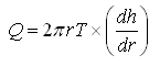                                                                                     (10.2) 

Eqn. (10.2) can be rearranged as follows: 

                                                                                         (10.3)

 

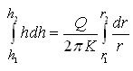
Let’s consider that two observation wells are installed in the aquifer at distances r₁ and r₂ from the pumping well, respectively with hydraulic heads h₁ and h₂ (Fig. 10.2). Now, integrating Eqn. (10.3) with these boundary conditions, we have:

 

                                        

 

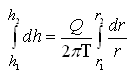
                                          (10.4)

         

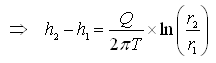
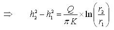
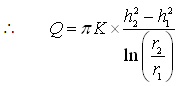
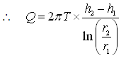                                                     (10.5)

 

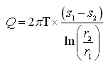
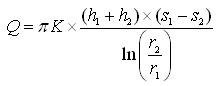
In practice, instead of the hydraulic head (h), drawdown (s) is measured, and hence after expressing h₁ and h₂ as drawdowns, Eqn. (10.5) can be written as:

 

                                                                                   (10.6)

 

Where, s₁ and s₂ are steady drawdowns in the two observation wells located respectively at r₁ and r₂ distances from the pumping well.

 

Eqn. (10.5) or (10.6) is known as the Thiem equation or equilibrium equation for confined aquifers. It is evident from the Thiem equation that the drawdown varies with the logarithm of the distance from the pumping well. Thiem equation can be used to compute constant pumping rate (Q), steady drawdown (s₁ or s₂) or distance of the point of observation from the pumping well (r₁ or r₂) if the aquifer parameter T and other variables are known. Additionally, this equation can also be used to calculate aquifer parameter T (or, K if the aquifer thickness is given) if other variables are known. Note that Eqn. (10.5) or (10.6) does not contain aquifer storage parameter (S); this is due to the fact that under steady-state conditions, there is no change in hydraulic head with time which means water is not coming from the aquifer storage.

 

Furthermore, if we consider that the first observation well is located at a distance r_w (radius of the pumping well) where hydraulic head is h_w and instead of the second observation well at r₂, we consider that r₂ = R₀ (radius of influence) where drawdown (s₂) is zero and hence hydraulic head is h₀ (static or pre-pumping groundwater level), the Thiem equation can be expressed as follows:

 

Eqn. (10.5) becomes 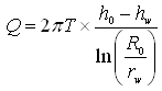                                                  (10.7)

 

and Eqn. (10.6) becomes 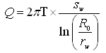                                                      (10.8)

 

Where, s_w denotes the drawdown in the aquifer at a distance r_w (i.e., at the well face). Since the pumping well is assumed to be 100% efficient (ideal condition), well losses can be neglected which enables us to take the drawdown in a pumping well equal to the drawdown at the well face (s_w).

 

The above form of the Thiem equation [Eqn. (10.7) or (10.8)] is practically very useful because unlike the earlier form of this equation [Eqn. (10.5) or (10.6)], it requires only one observation well’s data. Also, Eqn. (10.7) or (10.8) facilitates to determine radius of influence (R₀) of the well.

 

Finally, it is worth mentioning that drawdown changes gradually with time and equilibrium (steady-state) condition rarely exists under real field conditions. Therefore, when the difference in drawdowns (s₁-s₂) becomes essentially constant while both values are still increasing, it is assumed to be quasi-steady- state condition. Thus, the Thiem equation generally gives good results after only a few days of pumping.

 

10.2.5 Steady Radial Flow in Unconfined Aquifers

As we know that the analysis of flow in unconfined aquifers is more complicated than that in confined aquifers. Thiem also derived an equation for steady radial flow in unconfined aquifers which is discussed in this section. Besides the basic assumptions and the assumptions of radial symmetry and steady-state condition mentioned above, the following additional assumptions are made in this case:

       (1)       The aquifer is unconfined and underlain by a horizontal confining layer.

       (2)       The well is pumped at a constant rate.

       (3)       The Dupuit-Forchheimer assumptions are valid.

 

Using the Darcy’s law, the radial flow in the unconfined aquifer (Fig. 10.3) can be described as:

         

                                                                                 (10.9)

 

Where, Q = Constant rate of pumping, r = radial distance from the circular section to the pumping well, h = saturated thickness of the unconfined aquifer, K = hydraulic conductivity of the unconfined aquifer, and dh/dr = hydraulic gradient.

 

Arranging Eqn. (10.9), we have:

 

                                                                                              (10.10)

 

 

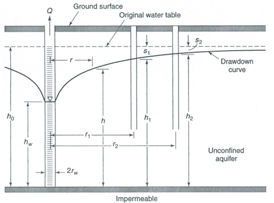
Fig. 10.3. Steady flow to a pumping well in an unconfined aquifer.

(Source: Todd, 1980)

 

Let’s consider that two observation wells are located in the unconfined aquifer at distances r₁ and r₂, with hydraulic heads h₁ and h₂, respectively (Fig. 10.3). Now, Eqn. (10.10) can be integrated with these boundary conditions as:

 

                                                                                    (10.11)

                                   

                                                                            (10.12)

 

Like the Thiem equation for confined aquifers, Eqn. (10.12) can also written in the form of drawdowns as follows: 

                                      (10.13)

 

Where, s₁ and s₂ are steady drawdowns in the two observation wells located respectively at r₁ and r₂ distances from the pumping well.

 

Eqn. (10.12) or (10.13) is called Thiem equation for unconfined aquifers or Dupuit’s equation. Like the Thiem equation for confined aquifers, this equation [Eqn. (10.12) or (10.13)] can also be used to compute Q, steady drawdowns (s₁ or s₂), distance of the point of observation from the pumping well (r₁ or r₂), or K depending on the known variables and parameters. 

Note that Eqn. (10.12) or (10.13) fails to describe accurately the drawdown curve near the pumping well because the large vertical flow components contradict the Dupuit-Forchheimer assumptions. However, the estimates of K for given hydraulic heads are good. In practice, the values of drawdowns should be small compared to the saturated thickness of the unconfined aquifer so as to ensure reliable use of Eqn. (10.12) or (10.3). To assess this condition, the ratio  (where s_max is the maximum drawdown in the unconfined aquifer and h₀ is the initial saturated thickness of the unconfined aquifer) is used. Two cases can arise, which are described below.

 

Case A: If  is less than or equal to 0.02, the drawdown in the unconfined aquifer can be considered very small compared to its thickness. In this case, Eqn. (10.12) or (10.13) can be used reliably. Alternatively, even the original Thiem equation [Eqn. (10.5), (10.6), (10.7) or (10.8)] can be used without significant errors. While applying Eqn. (10.5), (10.6), (10.7) or (10.8) to the unconfined aquifer problems, T is replaced with Kh₀ and the remaining variables/parameters are treated in the same manner as in case of confined aquifers.

 

Case B: If   is greater than 0.02, the drawdown in the unconfined aquifer is considered appreciable compared to its thickness. In this case also, the original Thiem equation [Eqn. (10.6) or (10.8)] can be used, but the observed drawdowns of the unconfined aquifer need to be corrected so that they can be representative for the equivalent confined aquifer. The following formula is used to correct the drawdowns of the unconfined aquifer:

 

                                            (10.14)

 

Where, s’ = correc^{ted drawdown (drawdown for the equivalent confined aquifer), s = drawdown observed in the unconfined aquifer, and h₀ = initial saturated thickness of the unconfined aquifer.}

 

^{Thus, using the corrected drawdowns, the original Thiem equation [Eqn. (10.6) or (10.8)] can be reliably applied to solve unconfined aquifer problems. Note that in this case, if one wishes to apply the} Dupuit’s equation for unconfined aquifers [i.e., Eqn. (10.13)], h₁ and h₂ of Eqn. (10.13) have to be replaced with (h₀-s₁) and (h₀-s₂), respectively. Thus, Eqn. (10.13) becomes:

 

                    (10.15) 

It is clear that Eqn. (10.15) is similar to Eqn. (10.6), if T of Eqn. (10.6) is replaced with Kh₀ and s₁ and s₂ of Eqn. (10.6) are replaced with ‘’ and ‘’, respectively according to Eqn. (10.14). Thus, the use of the original Thiem equation [Eqn. (10.6) or (10.8)] for solving unconfined aquifer problems even in the situation when drawdowns are considerably large is correct and justified provided that the observed drawdowns are corrected according to Eqn. (10.14).

 

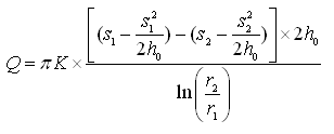
Moreover, if the drawdown in the unconfined aquifer is to be calculated/predicted using the original Thiem equation [Eqn. (10.6) or (10.8)], firstly drawdown at a given location is calculated assuming that the aquifer is confined. Thereafter, the calculated drawdown () is corrected using the following equation to obtain the actual drawdown (s) in the unconfined aquifer: 

                                                                             (10.16)

10.3 Steady Flow to Partially Penetrating Wells

10.3.1 What is a Partial Penetrating Well?

A well (pumping well or observation well) having screen length less than the aquifer thickness is known as a partially penetrating well. The flow pattern to such wells significantly differs from the flow pattern around the fully penetrating wells.

 

In many cases, the open hole or the well screen of a pumping/observation well does not extend from the top to the bottom of an aquifer. In all of the cases considered earlier, it was assumed that the well penetrates the entire saturated thickness of the aquifer. This causes flow in the aquifer to be essentially horizontal. However, the flow towards a partially penetrating well is three dimensional because of vertical flow components near the well (Fig. 10.4).

 

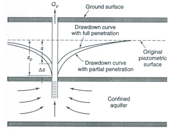
Fig. 10.4. Effect of a partially penetrating well on drawdown.

(Source: Todd, 1980)

 

10.3.2 Effect of Partially Penetrating Wells

It is obvious from Fig. 10.4 that the average length of flow lines into a partially penetrating well exceeds that into a fully penetrating well. Therefore, a greater resistance to flow is encountered, which results in increased drawdowns. In addition, if the aquifer is anisotropic, the values of the vertical hydraulic conductivity (K_v) and the horizontal hydraulic conductivity (K_h) are important. This will affect both the amount of water pumped from the well and the potential field caused by drawdown. For practical purposes, the following relationships exist between two similar wells - one partially penetrating and another fully penetrating the same aquifer:

 

If Q_p = Q, then  s_p > s                                     (10.17)

 

and                       if s_p = s, then Q_p < Q                                       (10.18)

 

Where, Q = well discharge, s = well drawdown, and the subscript ‘p’ refers to the partial penetrating well.

 

Detailed methods for analyzing the effects of partial penetration on well flow for steady and transient conditions in confined, leaky confined, unconfined, and anisotropic aquifer systems are presented by Hantush (1966), Hantush and Thomas (1966) and others. The calculation of steady drawdowns due to the pumping of partially penetrating wells in homogeneous and isotropic confined and unconfined aquifer systems is discussed in the subsequent section.

 

10.3.3 Partially Penetrating Well in Confined Aquifers

The drawdown (s_p) at the well face of a partially penetrating well in a confined aquifer is expressed as (Todd, 1980): 

                                               (10.19)

 

Where, s = drawdown with full penetration, and Ds = additional drawdown due to the partial penetration. Note that here the value of s can be calculated using the Thiem equation described above.

 

For steady-state flow towards a well in a confined aquifer with the screen starting from the top of the aquifer as shown in Fig. 10.5(a), the additional drawdown due to the partial penetration (Ds) can be given as (Todd, 1980): 

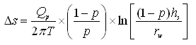                            (10.20)

Where, T = aquifer transmissivity, p = penetration fraction (i.e., p = h_s/b), h_s = screen length, and r_w = radius of the well.

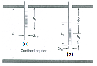
 Fig. 10.5. Two basic configurations of well screen. (Source: Todd, 1980)

 

Equation (10.20) is valid for p > 0.20. Note that the increase in drawdown is the same whether the screen of a partially penetrating well starts from the top or from the bottom of the aquifer (Todd, 1980).

 

On the other hand, for the case of a well installed in a confined aquifer with the screen located in the center of the aquifer thickness [Fig. 10.5(b)], the value of Ds is given as (Todd, 1980): 

                                                                  (10.21)

 

10.3.4 Partially Penetrating Well in Unconfined Aquifers

The drawdown (s_p) at the well face of a partially penetrating well in an unconfined aquifer can be expressed as (Todd, 1980): 

                                                                      (10.22)

 

Where, h₀ = initial saturated thickness of the unconfined aquifer. In this case also, the value of s can be calculated using the Thiem equation described above.

 

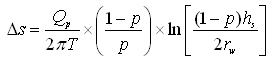
For a partially penetrating well in an unconfined aquifer with the well screen location as shown in Fig. 10.5(a), Eqn. (10.20) can be modified as follows (Todd, 1980):

 

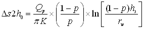                        (10.23)

 

Where, h₀ = initial saturated thickness of the unconfined aquifer, and K = T/h₀.

Similarly, Eqn. (10.21) can be modified for a partially penetrating well in an unconfined aquifer with the screen located in the center of the aquifer thickness as follows (Todd, 1980):

 

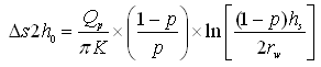                        (10.24)

 

Given the values of s and Ds2h₀, the drawdown (s_p) at the well face of a partially penetrating well in an unconfined aquifer can be calculated using Eqn. (10.22).

 

10.3.5 Tips for Handling Partial Penetration Problem

Although the evaluation of the effects of partial penetration is complicated except for the simplest cases, common field situations often reduce the practical importance of partial penetration. For example, any well with 85% or more open or screened hole in the saturated aquifer thickness may be practically considered as fully penetrating (Todd, 1980). If an observation well fully penetrates an anisotropic aquifer, or if a partially penetrating observation well is located at a distance greater than from the pumping well, the effect of a partially penetrating pumping well is negligible (Hantush, 1964). However, if the pumping well is partially penetrating, and the observation wells are also partially penetrating and located closer to the pumping well than, then the drawdown formula is different and highly complex. Hantush (1961, 1964) analyzed the drawdown behavior in such observation wells and provided analytical solutions for some specific cases. Further, the effects of partial penetration of a well pumping from an unconfined aquifer are discussed in Neuman (1974).

 

Moreover, for the many alluvial aquifer systems having pronounced anisotropy, the vertical flow component becomes very small. Hence, a partially penetrating pumping well can be approximated as a fully penetrating well in a confined or leaky confined aquifer with a saturated thickness equal to the length of the well screen (Todd, 1980).

 

10.4 Steady Flow to Cavity Wells

Cavity well is a special type of tubewell constructed in the confined aquifer, which has no strainer. It draws water through the cavity formed in the aquifer just below the upper confining layer of the confined aquifer (Fig. 10.6). It is not very deep and requires a thick clay layer (or, rock) just above the aquifer layer to form a strong and reliable roof above the cavity. The hydraulics of cavity wells under steady-state conditions was developed by Mishra et al. (1970) and is described in Michael and Khepar (1999).  

 

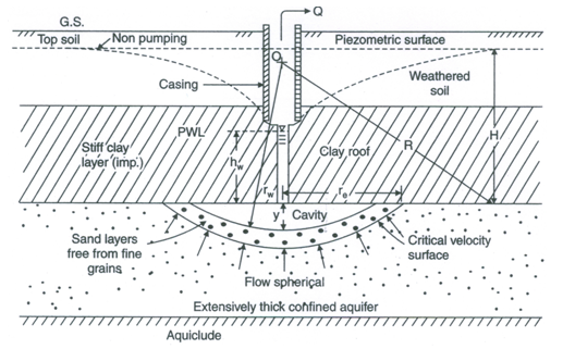
Fig. 10.6. Schematic diagram of a cavity well subject to pumping.

(Source: Raghunath, 2007)

Assuming the cavity to be segment of a sphere of radius r_w resting on the top of a homogeneous and isotropic confined aquifer of infinite areal extent and extensive thickness, the discharge of the cavity well under steady flow conditions is given as (Raghunath, 2007): 

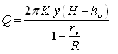                                        (10.25)

 

Where, Q = constant rate of pumping (well discharge), K = hydraulic conductivity of the confined aquifer, y = depth of the cavity at the center, H = initial/pre-pumping hydraulic head (or, hydraulic head at radius of influence), R = radius of influence of the cavity well, and h_w = hydraulic head at a distance r_w (radius of the cavity).

 

Further, the width of the cavity (r_e) is given as (Raghunath, 2007): 

                                              (10.26)

 

References

Hantush, M.S. (1961). Aquifer test on partially penetrating wells. Proceedings of the American Society of Civil Engineers, ASCE, 87: 171-195. 

Hantush, M.S. (1964). Hydraulics of wells. In: V.T. Chow (Editor), Advances in Hydroscience, Volume 1, pp. 281-432, Academic Press, New York.

Hantush, M.S. (1966). Wells in homogeneous anisotropic aquifers. Water Resources Research, 2: 273-279.

Hantush, M.S. and Thomas, R.G. (1966). A method for analyzing a drawdown test in anisotropic aquifers. Water Resources Research, 2: 281-285.

Michael, A.M. and Khepar, S.D. (1999). Water Well and Pump Engineering. Tata McGraw-Hill Publishing Co. Ltd., New Delhi.

Mishra, A.P., Anjaneyulu, B. and Lal, R. (1970). Design of cavity wells. Journal of Agricultural Engineering, ISAE, 8: 12-15.

Neuman, S.P. (1974). Effect of partial penetration on flow in unconfined aquifers considering delayed gravity response. Water Resources Research, 10: 303-312.

Raghunath, H.M. (2007). Ground Water. New Age International (P) Limited, New Delhi.

Roscoe Moss Company (1990). Handbook of Ground Water Development. John Wiley & Sons, New York.

Todd, D.K. (1980). Groundwater Hydrology. John Wiley and Sons, New York.

 

Suggested Readings

Todd, D.K. (1980). Groundwater Hydrology. John Wiley & Sons, New York.

Fetter, C.W. (2000). Applied Hydrogeology. Fourth Edition. Prentice Hall, NJ.

Michael, A.M. and Khepar, S.D. (1999). Water Well and Pump Engineering. Tata McGraw-Hill Publishing Co. Ltd., New Delhi.

Sarma, P.B.S. (2009). Groundwater Development and Management. Allied Publishers Pvt. Ltd., New Delhi.

Raghunath, H.M. (2007). Ground Water. New Age International (P) Limited, New Delhi.