Ground Water, Wells and Pumps

Lesson 12 Determination of Aquifer Parameters

12.2 Laboratory Methods

12.2.1 Grain-Size Analysis (GSA) Method

Hydraulic conductivity of the aquifer material is related to its grain/particle size. Grain-size analysis (GSA) method is based on predetermined relationships between an easily determined soil property (e.g., texture, pore-size distribution, grain-size distribution, etc.) and the hydraulic conductivity (K). In general, the permeability of porous subsurface formations appears to be proportional to some mean grain diameter squared, which reflects the size of a pore, along with the spread or distribution of grain/particle sizes. Determination of hydraulic conductivity from the grain-size analysis of geologic samples (aquifer or non-aquifer materials) is useful, especially during the initial stage of many groundwater studies such as designing aquifer tests or any preliminary studies when the field measured aquifer hydraulic conductivity is not available.

 

Grain-size analysis method involves the collection of geologic samples from the field during test drilling or well drilling and their sieve analysis in the laboratory. The collected geologic samples are subjected to sieve analysis by using a set of standard sieves and the results of sieve analysis are expressed as the weight percentage passing (or percentage finer than) the mesh size of each sieve. These data are used to construct a grain-size distribution curve (also known as ‘particle-size distribution curve’) for a given geologic sample. Grain-size distribution curve is constructed by plotting grain/particle sizes on the logarithmic scale on X-axis) and percentage finer by weight on the arithmetic scale on Y-axis as shown in Fig. 12.1. From this curve, one can obtain grain-size values at different values of percent finer; for example, the grain-size value at 10% (denoted by D₁₀) which is called ‘effective grain size’ or the grain-size value at 50% (denoted by D₅₀) which is called ‘mean grain size’.

 

Several formulae, varying from very simple to complex, based on analytic or experimental work have been developed for the estimation of K from the grain-size distribution data; for example, Hazen formula,  Harleman formula, Shepherd formula, Kozeny-Carman formula, Alyamani and Sen formula, etc. (Freeze and Cherry, 1979; Batu, 1998). Of these formulae, the Hazen formula is a simple relationship between the hydraulic conductivity (K) and the effective grain size (or diameter), and it is often used in groundwater hydrology for the estimation of hydraulic conductivity from grain-size distribution data. It is given as (Freeze and Cherry, 1979):

 

                                                K = A × D₁₀²                                                 (12.1)

 

Where, K = hydraulic conductivity, (cm/s); D₁₀ = effective grain diameter, (mm) which is determined from the grain-size distribution curve (Fig. 12.1); and A = constant, which is usually taken as 1.0 (Freeze and Cherry, 1979).

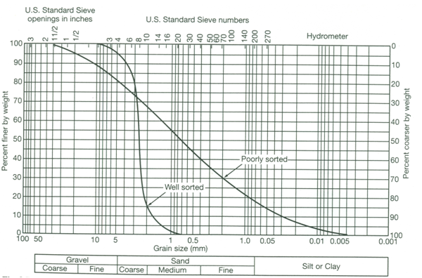
Fig. 12.1. Grain-size distribution curves for well sorted and poorly sorted samples. (Source: Brassington, 1998)

 

The advantage of the GSA method is that an estimate of the K value is often simpler and faster than its direct determination. However, the major drawback of the method is that the empirical relationship may not be accurate in all cases, and hence may be subject to random errors.

 

12.2.2 Permeameter Methods

In the laboratory, hydraulic conductivity of undisturbed geologic samples or soil samples can be determined in the laboratory by a permeameter. The permeameter methods essentially provide saturated hydraulic conductivity. If undisturbed geologic samples can be collected from shallow aquifers or confining layers using a core sampler, these samples can be used to determine the saturated hydraulic conductivity of aquifer or non-aquifer materials in the laboratory in the same way as undisturbed soil samples. In permeameters, flow is maintained through a small sample of material while the measurements of flow rate and head loss are made. The constant-head and falling-head types of permeameters (Fig. 12.2) are simple to operate and widely used.

 

The constant-head permeameter [Fig. 12.2(a)] can measure hydraulic conductivities of consolidated or unconsolidated formations under low heads.

Water enters the medium cylinder from the bottom and is collected as overflow after passing upward through the material. From the Darcy’s law, the hydraulic conductivity (K) can be expressed as:

 

                                                  (12.2)

 

Where, V = flow volume collected during time t, A = cross-sectional area of the sample, L = length of the sample, and h = constant head applied to the sample.  

 

It is important that the sample be thoroughly saturated to remove entrapped air. Several different heads in a series of tests provide a reliable measurement.

 

A second procedure utilizes the falling-head permeameter as shown in Fig. 12.2(b). In this case, water is added to the tall tube; it flows upward through the cylindrical sample and is collected as overflow. The test consists of measuring the rate of fall of the water level in the tube. The hydraulic conductivity (K) can be obtained by noting that the flow rate in the tube must equal that through the sample. Flow rate in the tube (Q) is given as: 

 

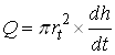                                            (12.3)

 

and the flow rate through the sample is given by Darcy’s law as:

 

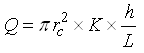                                    (12.4)

 

 

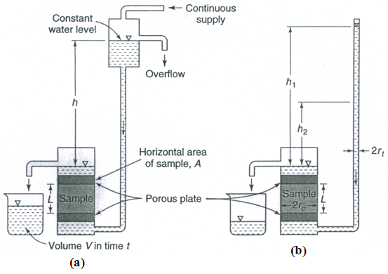
 Fig. 12.2. Permeameters for measuring saturated hydraulic conductivity of geologic or soil samples: (a) Constant-head permeameter; (b) Falling-head permeameter. (Source: Mays, 2012)

 

After equating Eqns. (12.3 and 12.4) and integrating, we have:

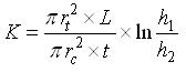                                                  (12.5)

 

Where L, r_t, and r_c are shown in Fig. 12.2b, and t is the time interval for the water level in the tube to fall from h₁ to h₂.

 

Permeameter results may bear little relation to actual field hydraulic conductivities. Undisturbed samples of the unconsolidated subsurface formation (aquifer or non-aquifer material) are difficult to obtain, while disturbed samples are not representative of actual field conditions because they experience changes in porosity, packing, and grain orientation, which modify hydraulic conductivities. Note that one or even several samples from an aquifer may not represent the overall hydraulic conductivity of an aquifer. Variations of several orders of magnitude frequently occur for different depths and locations in an aquifer (Todd, 1980). Also, directional properties of hydraulic conductivity cannot be recognized by the laboratory methods.

 

12.3 Field Methods

12.3.1 Tracer Test

Field determination of hydraulic conductivity can be made by measuring the time interval for a water tracer to travel between two observation wells or test holes. For the tracer, a dye such as sodium fluorescein, or a salt such as calcium chloride is convenient, inexpensive, easy to detect and safe. Fig. 12.3 shows the cross section of a portion of an unconfined aquifer with groundwater flowing from Hole A toward Hole B. The tracer is injected as a slug in Hole A, after which water samples are taken from Hole B to determine the time taken by the tracer to reach Hole B. As the tracer flows through the aquifer with an average interstitial velocity or seepage velocity (V_s), V_s needs to be computed and it is given as follows:

                                              (12.6)

 

Where, K = hydraulic conductivity of the aquifer, n_e = effective porosity of the aquifer, h = head difference between the two holes/observation wells (Fig. 12.3), and L = distance between the two holes/observation wells (Fig. 12.3). 

However, V_s can also be calculated as: 

                                                      (12.7)

 

Where, t is the time taken by the tracer to travel from Hole A to Hole B.

  

Fig. 12.3. Illustration of a tracer test in an unconfined aquifer for determining hydraulic conductivity. (Source: Mays, 2012)

 

Equating Eqns. (12.6) and (12.7) and solving for K yields: 

                                                       (12.8)

 

Although the tracer test is simple in principle, its results are only approximations because of serious constraints in the field. Therefore, this test should be conducted considering the following limitations (Todd, 1980):

(1)    The holes/observation wells need to be close together; otherwise, the travel time interval can be excessively long.

(2)    Unless the flow direction is accurately known, the tracer may miss the downstream hole entirely. In this case, multiple sampling holes can help, but it will increase the cost and complexity of conducting the tracer test.

(3)    If the aquifer is stratified with layers with differing hydraulic conductivities, the first arrival of the tracer will result in the hydraulic conductivity considerably larger than the average hydraulic conductivity of the aquifer.

 

 An alternative tracer technique, which has been successfully applied under field conditions, is the point dilution method (Todd, 1980). In the point dilution method, a tracer is introduced into an observation well and thoroughly mixed with the groundwater present in the observation well. Thereafter, as water flows into and from the well, repeated measurements of tracer concentration are made. Using these data, a dilution curve is plotted. The groundwater velocity can be obtained from the analysis of the dilution curve. Using the groundwater velocity, measured water-table gradient and Darcy’s law, we can obtain a localized estimate of the aquifer hydraulic conductivity as well as the direction of groundwater flow.

 

Example Problem:

A tracer test was conducted in an unconfined aquifer to determine its hydraulic conductivity. For this, two observation wells were installed 30 m apart and the hydraulic heads at these two locations were measured as 20.5 m and 18.4 m, respectively. During the test, it was found that the tracer injected in the first observation well arrived at the second observation well in 180 hours. If the effective porosity of the aquifer is 18%, calculate the hydraulic conductivity of the unconfined aquifer.

 

Solution:

Given:  Hydraulic head difference between the two observation wells (h) = 20.5 m – 18.4 m = 2.1 m, distance between the two observation wells (L) = 30 m, effective porosity (n_e) of the aquifer = 18% = 0.18, and the time taken by the tracer to travel a distance of L (t) = 180 h = 180¸24 = 7.5 days.

 

Using Eqn. (12.8) for computing the hydraulic conductivity of the aquifer (K) and substituting the above values, we have: 

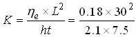 =10.29 m/day, Ans.

 

12.3.2 Auger-Hole Method

The auger-hole method involves the measurement of the change in water level after the rapid removal of a volume of water from an unlined cylindrical hole. If the soil is loose, a screen may be necessary to maintain the test-hole geometry. The method is relatively simple and is most adapted to shallow water-table conditions. The value of hydraulic conductivity (K) obtained is essentially horizontal hydraulic conductivity (K_h) in the immediate vicinity of the test hole. 

Figure 12.4 illustrates an auger hole and the dimensions required for the computation of hydraulic conductivity. The hydraulic conductivity is given as (Todd, 1980):

 

                                          (12.9)

 

Where  is the measured rate of rise in cm/s and the factor 864 yields K values in m/day. The factor C is a dimensionless constant governed by the variables shown in Fig. 12.4 and its value can be obtained from the standard table given in Todd (1980) or Mays (2012).

 

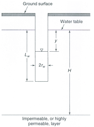
 Fig. 12.4. Schematic of an auger hole and its dimensions for determining aquifer hydraulic conductivity. (Source: Mays, 2012)

 

Several other techniques similar to the auger-hole method have been developed in which water level changes are measured after an essentially instantaneous removal or addition of a volume of water. With a small-diameter pipe driven into the ground, K can be found by the piezometer method, or tube method (van Schilfgaarde, 1974).

 

12.3.3 Slug Test

Pumping tests are typically expensive to conduct because of the installation costs of wells. Where a pumping test cannot be conducted, the slug test serves as an alternative approach for determining aquifer parameters. However, the aquifer parameters obtained by slug tests are representative of a smaller area (the area in the vicinity of the well in which slug tests are conducted). Nevertheless, slug test has been used for several years as a cost-effective and quick method of estimating the hydraulic properties of confined and unconfined aquifers. More recently (since the 1980s) it has gained even more popularity in: (i) obtaining estimates of hydraulic properties of contaminated aquifers where treating the pumped water is not desirable or feasible, and (ii) field investigations of  low-permeability materials, particularly for studies of potential waste storage or disposal sites (Mays, 2012). The materials at these sites may have a hydraulic conductivity which is too low to be determined by pumping tests.

 

Slug test consists of measuring the recovery of head in a well after near instantaneous change in head at that well. A solid object (slug) is rapidly introduced into or removed from the well, causing a sudden change (increase or decrease) in the water level in the well. Tests can also be performed by introducing an equivalent volume of water into the well; or, an equivalent volume of water can be removed from the well, causing a sudden decrease in the water level. Following the sudden change in head, the water level returns to the static water level. While the water level is returning to the static level, the head is measured as a function of time (referred to as the response data). These response data are used to determine the hydraulic properties of the aquifer using one of several methods of analyses. Various methods have been developed for the analysis of slug-test data obtained from different slug-test designs in confined and unconfined aquifers. A comprehensive description about the methodology of slug tests and their data analysis can be found in Butler (1998), while a summary of slug tests and their applications is presented in Mays (2012) and Fetter (2000). 

 

12.3.4 Pumping Test

To date, pumping test is the most reliable method for determining aquifer hydraulic conductivity. In the pumping test designed for aquifer parameter determination, a pumping well is pumped and the resulting drawdown is measured in one or more observation wells located at varying distances from the pumping well (within its radius of influence). The time-drawdown data thus obtained at a given location are analyzed to determine hydraulic parameters of confined, unconfined and leaky aquifers. A properly designed pumping test can also yield the hydraulic parameters of leaky confining layers (aquitards). Thus, an integrated K value over a sizable aquifer section can be obtained by pumping tests. Unlike the laboratory methods, the aquifer is not disturbed by pumping test, and hence the reliability of pumping test is superior to the laboratory methods. The details of pumping test and the determination of aquifer parameters from pumping-test data analysis are given in Lessons 13 and 14, respectively.

 

References

Batu, V. (1998). Aquifer Hydraulics: A Comprehensive Guide to Hydrogeologic Data Analysis. John Wiley & Sons, New York.

Brassington, R. (1998). Field Hydrogeology. Second Edition, John Wiley & Sons, Chichester, England.

Butler, J.J., Jr. (1998). The Design, Performance, and Analysis of Slug Tests. Lewis Publishers, Boca Raton, Florida.

Fetter, C.W. (2000). Applied Hydrogeology. Fourth Edition. Prentice Hall, NJ.

Freeze, R.A. and Cherry, J.A. (1979). Groundwater. Prentice-Hall, Englewood Cliffs, New Jersey.

Mays, L.W. (2012). Ground and Surface Water Hydrology. John Wiley and Sons, New York.

Todd, D.K. (1980). Groundwater Hydrology. John Wiley & Sons, New York.

van Schilfgaarde, J. (Editor) (1974). Drainage for Agriculture. Agronomy Monograph  No. 17, American Society of Agronomy, Madison, Wisconsin.

 

Suggested Readings

Todd, D.K. (1980). Groundwater Hydrology. John Wiley & Sons, New York.

Raghunath, H.M. (2007). Ground Water. Third Edition, New Age International Publishers, New Delhi.

Sarma, P.B.S. (2009). Groundwater Development and Management. Allied Publishers Pvt. Ltd., New Delhi.