Ground Water, Wells and Pumps

Lesson 15 Well Interference and Multiple Well Systems

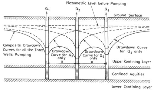
Fig. 15.1. Well interference in a well field having three pumping wells.   (Modified from Todd, 1980)

 

15.1.1 Well Interference in Confined Aquifer Systems

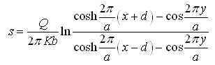
From the principle of superposition, the drawdown at any point in the area of influence caused by the pumping of several wells is equal to the sum of the individual drawdowns caused by each pumping well, which is mathematically expressed as follows (Todd, 1980):                                           

                                                                (15.1) 

Where, s = total drawdown at a given point due to the pumping of multiple wells, and s_a, s_b, s_c, …., s_n are individual drawdowns at the point caused by the pumping of wells a, b, c, …., n, respectively. 

15.1.2 Unconfined Aquifer and Well Interference

The linear superposition principle [Eqn. (15.1)] is valid only for confined aquifer systems, in which the value of aquifer transmissivity does not change with drawdown. In unconfined (water-table) aquifer systems, if the drawdown is significant compared to its initial saturated thickness, the use of linear superposition will result in a predicted composite drawdown that is less than the actual composite drawdown. As a decrease in the saturated thickness of an unconfined aquifer reduces the aquifer transmissivity, the multiple-well system in this aquifer will result in a composite hydraulic gradient greater than that of an equivalent confined system in order to compensate for a reduced value of aquifer transmissivity. Thus, when two or more wells are discharging groundwater from an unconfined aquifer with intersecting cones of depressions, the composite drawdown predicted by Eqn. (15.1) is always an estimate-in-error of the actual drawdown. Therefore, the following steps are followed to calculate the composite drawdown due to well interference in unconfined aquifers (Kasenow, 2001):

Step 1: Determine the theoretical confined drawdown (steady or unsteady) using known T (i.e., Kh₀) and S_y values for each production well as if they were pumping groundwater in isolation.

Step 2: Determine a resulting sum for these confined drawdowns.

Step 3: Correct this resulting sum to determine total unconfined drawdown at the observation point, which includes well interference drawdowns: 

                                                                               (15.2) 

Where, s = drawdown in the unconfined aquifer [L]; s’= drawdown in the equivalent confined aquifer [L], and h₀ = initial saturated thickness of the aquifer [L].

Step 4: Finally, to determine the dewatering component of the drawdown, subtract the result obtained in Step 2 from the result obtained in Step 3.

The above procedure is necessary to be followed while computing composite drawdown due to well interference in unconfined aquifer systems; otherwise a large error may occur (Kasenow, 2001).

 

15.2 Salient Applications of Well Interference

• In designing well-field layouts, it is necessary to take into account well interference. The water level in a well during pumping determines the length of suction pipe necessary to carry groundwater to the ground surface. The characteristics of the pump and the horsepower requirements of the motor also depend on the depth to the pumping level; considerably high energy is required for withdrawing groundwater from deeper depths.

• Generally, the well field designed for water supply purposes should be spaced as far apart as possible to minimize well interference, which in turn will minimize drawdowns. If wells are spaced too closely together, the amount of well interference could be very high.

• For drainage (or dewatering) wells, however, the well field is designed to increase well interference so as to enhance the drainage or dewatering effect.

• Aligning wells parallel to a line source of recharge (e.g., river, lake) would result in less well interference compared to a perpendicular configuration of wells. 

 

15.3 Analysis of Multiple Well Systems

As mentioned earlier, if there are several wells in a given well field, the drawdown at any point is the sum of the drawdowns due to individual pumping wells. The drawdown depends on the pumping pattern, i.e., number of pumping wells, their pumping rates and their arrangement. Solutions can be obtained using steady-state or unsteady (transient) flow equations depending on the field situation. Multiple well systems are used for lowering the groundwater level in a given area to facilitate subsurface drainage or excavation for foundation work, mining, etc. Steady-state solutions for multiple well systems are presented in this section for three major cases: (i) drawdown for the well systems parallel to a line source, (ii) well discharges for different well configurations, and (iii) required drawdown for the well systems used for dewatering.    

 

15.3.1 Well Systems Parallel to Line Source

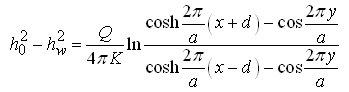
Wells may be closely spaced (resulting in well interference) and all the wells may be connected to a common supply pipe to meet the large demand of water supply. For an array of a number of equally-spaced fully penetrating wells, all discharging at the same rate, parallel to a line source (Fig. 15.2), steady drawdown in the confined aquifer at any point (x, y) is given as (Forchheimer, 1908 as referred in Raghunath, 2007): 

                                                     (15.3)

 

Where, s = steady drawdown at the observation point (x,y), [L]; a = spacing between the wells, [L]; Q = discharge of each well, [L³T^-1]; and d = distance of the observation point from the line source, [L].

 

For unconfined aquifers, Eqn. (15.3) is expressed as:

                                             (15.4)

 

Where, h_w= water level in the well during pumping from the well bottom [L].

 

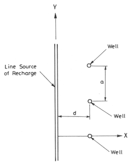
Fig. 15.2. Well parallel to a line source of recharge.

 

15.3.2 Well Discharge for Different Well Configurations

Muskat in 1973, as referred in Raghunath (2007), developed analytical solutions (Eqns. 15.5 to 15.7) for well discharges considering various well patterns localized near the centre of a well field of radius R₀ (i.e., radius of influence for each well) such that for each well the head at the external boundary can be taken to be  (Fig. 15.3). It was assumed that all the wells fully penetrate a confined aquifer, have the same diameter and drawdown, and discharge for the same period of time. Three configurations (linear, triangular and square) of closely spaced multiple wells as shown in Fig. 15.3 are discussed below as three cases. 

 

(1) Case 1: Discharge of the two wells spaced at a distance a (a  R₀)

 

For Confined Aquifers: 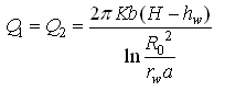                                        (15.5a)

 

Where, K = hydraulic conductivity of the aquifer [LT^-1]; H = head at external boundary (i.e., water level in the well before pumping from the bottom of the well) [L]; and H-h_w = s_w = drawdown of single well at a given discharge Q [L].

 

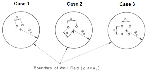
Fig. 15.3. Three configurations of wells closely spaced in a well field.

 

For Unconfined Aquifers:

Eqn. (15.5a) can also be applied to unconfined aquifers by replacing H with H²/2b and h_w with /2b (Raghunath, 2007), which results in:

 

                                                                          (15.5b)

 

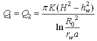
(2) Case 2: Discharge of the three wells spaced at a distance a (a  R₀)

 

For Confined Aquifers: 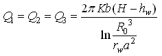                                 (15.6a)

 

For Unconfined Aquifers: 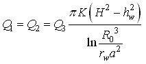                        (15.6b)

 

(3) Case 3: Discharge of the four wells spaced at a distance a (a  R₀)

 

For Confined Aquifers: 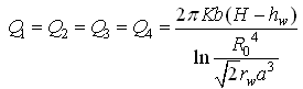                          (15.7a)

 

For Unconfined Aquifers: 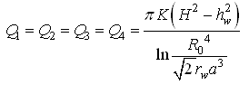             (15.7b)

 

Note that as the number of wells in the group increases, the mutual interference between wells becomes more, which results in the reduction of production capacity of individual wells.

 

15.3.3 Multiple Well Systems for Dewatering

Design of dewatering systems has great importance in drainage, mining and foundation engineering. It involves a number of pumping wells for accomplishing the dewatering objective. The principle of superposition is used to calculate drawdown and required well discharge. For a confined aquifer, the principle of superposition yields (Charbeneau, 2000):

                            

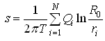                                                                                 (15.8)

 

Where, s = drawdown of the system of wells [L], Q_i = discharge from the i^th well [LT^-3], R₀ = radius of influence [L], and r_i = radius of the i^th well [L].

 

If the discharge from each well is the same, Eqn. (15.8) can be written as:

 

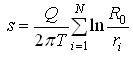                                                                                      (15.9)

 

Where, Q is the discharge from each well. Eqn. (15.9) is important because it indicates that with a multiple number of wells, all pumping at the same rate, the drawdown at any point depends only on the geometry of the system.

 

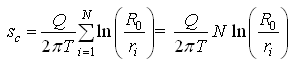
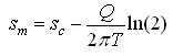
(1) Circular Well System

Jacob (1950) analyzed the dewatering problem with a number of pumping wells arranged in a circle as shown in Fig. 15.4. It was assumed that each well is pumping at the same rate. We are often interested in the drawdown at the centre of the system of wells, which might correspond to the centre of an excavation for example, and the drawdown at each of the wells and at midpoint between wells on the circle of the system.

 

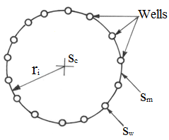
 Fig. 15.4. Geometry for a circular dewatering system.

 

• For the drawdown at the centre of the system of wells, the radii from each of the wells to the centre (r_i) are the same (Fig. 15.4). Thus, Eqn. (15.9) can be written as (Charbeneau, 2000): 

                                                      (15.10)

 

Where, s_c = drawdown at the center of the system of wells [L]. 

• For the drawdown at each well, Eqn. (15.9) becomes:     

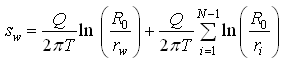                                                        (15.11)

 

Where, s_w = drawdown at each well [L], and r_w = radius of each well [L]. 

Jacob (1950) used several trigonometric identities to demonstrate that Eqn. (15.11) reduces to:

 

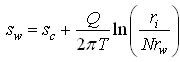                                                                       (15.12)

 

• For the drawdown at midpoint between the wells, Eqn. (15.9) becomes: 

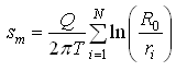                                        (15.13)

 

Where, s_m = drawdown at midpoint between the wells [L]. 

Again, using trigonometric identities, it can be shown that Eqn. (15.13) reduces to:

 

                                                                                (15.14)

 

It should be noted that s_w > s_c > s_m.   

 

(2) Linear Well System

For a linear well system, let’s consider a line of wells with a constant well spacing of a and the number of wells in the line N (Fig. 15.5). The number of wells (N), well spacing (a), and the length of line (L) are related as N = L/a so that the length of the line is considered to extend a distance a/2 beyond the last well at each end. We are usually interested to find out the drawdown at an arbitrary point away from the line of wells (Charbeneau, 2000).

 

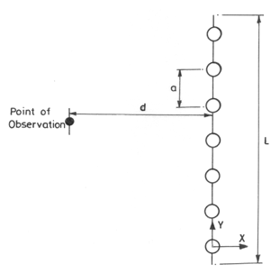
Fig. 15.5. Geometry for a linear dewatering system.

 

The drawdown at any arbitrary distance d from one end of the row (chosen as the origin) satisfies Eqn. (15.9), and we have the following expression for confined aquifer systems (Charbeneau, 2000):                  

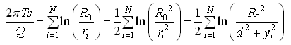          (15.15)               

The summation can be approximated by the integral because both are equal to N as   . Thus, we have:

 

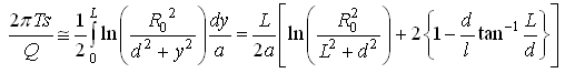         (15.16)     

 

As L/a = N and NQ = Q_T, Eqn. (15.16) can be written as: 

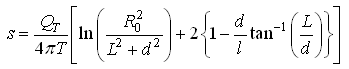                                          (15.17) 

                  

Where, Q_T = total discharge [LT^-3]. 

Similarly, for unconfined aquifer systems, we have:

 

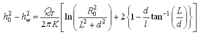                                          (15.18)

 

References

Charbeneau, R.J. (2000). Groundwater Hydraulics and Pollutant Transport. Prentice-Hall, Englewood Cliff, NJ.

Jacob, C.E. (1950). Flow of Groundwater. In: H. Rouse (Editor), Engineering Hydraulics, Chapter 5, pp. 321-386, Wiley, New York.

Kasenow, M. (2001). Applied Groundwater Hydrology and Well Hydraulics. Second Edition, Water Resources Publications, Highlands Ranch, Colorado.

Raghunath, H.M. (2007). Ground Water. Third Edition, New Age International Publishers, New Delhi.

Todd, D.K. (1980). Groundwater Hydrology. John Wiley and Sons, New York.

 

Suggested Readings

Todd, D.K. (1980). Groundwater Hydrology. John Wiley & Sons, New York.

Raghunath, H.M. (2007). Ground Water. Third Edition, New Age International Publishers, New Delhi.

Sarma, P.B.S. (2009). Groundwater Development and Management. Allied Publishers Pvt. Ltd., New Delhi.

Charbeneau, R.J. (2000). Groundwater Hydraulics and Pollutant Transport. Prentice-Hall, Englewood Cliff, NJ.