Electrical M/C's and Power Utilization

LESSON 21. DC motor speed control methods-field and armature control

Speed control by varying armature resistance

The inherent armature resistance r_a being small, speed n versus armature current I_a characteristic will be a straight line with a small negative slope as shown in figure 8.14 . At no load (i.e., I_a = 0) speed is highest and . Note that for shunt motor, voltage applied to the field and armature circuit are same and equal to the supply voltage V. However, as the motor is loaded, I_ar_a drop increases making speed a little less than the no load speed n_o. For a well designed shunt motor this drop in speed is small and about 3 to 5% with respect to no load speed. This drop in speed from no load to full load condition expressed as a percentage of no load speed is called the inherent speed regulation of the motor. It is for this reason, a d.c shunt motor is said to be practically a constant speed motor (with no external armature resistance connected) since speed drops by a small amount from no load to full load condition.

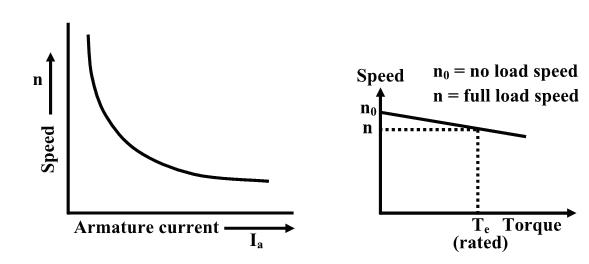
Fig. 8.14  Characteristics of shunt motor

Since T_e = kjI_a, for constant j  operation, T_e becomes simply proportional to I_a. Therefore, speed vs. torque characteristic is also similar to speed vs. armature current characteristic as shown in figure.

The slope of the n vs I_a or n vs T_e characteristic can be modified by deliberately connecting external resistance r_ext in the armature circuit. One can get a family of speed vs. armature curves as shown in figures 8.15.  for various values of r_ext. From these characteristic it can be explained how speed control is achieved. Let us assume that the load torque T_L is constant and field current is also kept constant. Therefore, since steady state operation demands T_e = T_L,and T_e = kjI_a too will remain constant; which means I_a will not change. Suppose r_ext = 0, then at rated load torque, operating point will be at C and motor speed will be n. If additional resistance r_ext1 is introduced in the armature circuit, new steady state operating speed will be n₁ corresponding to the operating point D. In this way one can get a speed of n₂ corresponding to the operating point E, when r_ex2t is introduced in the armature circuit. This same load torque is supplied at various speeds. Variation of the speed is smooth and speed will decrease smoothly if r_ext is increased. Obviously, this method is suitable for controlling speed below the base speed and for supplying constant rated load torque which ensures rated armature current always. Although, this method provides smooth wide range speed control (from base speed down to zero speed), it has a serious draw back since energy loss takes place in the external resistance r_ext reducing the efficiency of the motor.

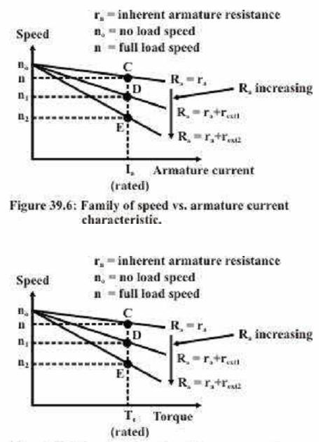
Fig. 8.15  Family of speed vs Torque and speed vs current characteristic,

Speed control by varying field current

In this method field circuit resistance is varied to control the speed of a d.c shunt motor. Let us rewrite .the basic equation to understand the method.

If we vary I_f, flux j will change, hence speed will vary. To change I_f, an external resistance is connected in series with the field windings. The field coil produces rated flux when no external resistance is connected and rated voltage is applied across field coil. It should be understood that we can only decrease flux from its rated value by adding external resistance. Thus the speed of the motor will rise as we decrease the field current and speed control above the base speed will be achieved. Speed versus armature current characteristic is shown in figure 8.15  for two flux values j and j₁. Since j₁ < j, the no load speed n₀’ for flux value j₁ is more than the no load speed n₀ corresponding to j. However, this method will not be suitable for constant load torque. To make this point clear, let us assume that the load torque is constant at rated value. So from the initial steady condition, we have T_Lrated = T_el = kjI_arated . If load torque remains constant and flux is reduced to j₁, new armature current in the steady state is obtained from kj₁I_al=T_Lrated. Therefore new armature current is

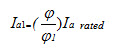
But the fraction ; hence new armature current will be greater than the rated armature current and the motor will be overloaded. This method therefore, will be suitable for a load whose torque demand decreases with the rise in speed keeping the output power constant as shown in figure 8.16. Obviously this method is based on flux weakening of the main field. Therefore at higher speed main flux may become so weakened, that armature reaction effect will be more pronounced causing problem in commutation.

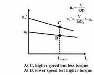
Fig. 8. 16 Family of speed vs armature current characteristics