System Engineering

LESSON 2. Linear Growth Model

Assumption of the model:

In linear growth model, we make the assumption  on crop growth system that the crop will grow during the crop period i.e. as the day’s increase the crop will grow.

i.e.       ∆W  ∆t.

Construction of the model:

            ∆W  ∆t

            ∆W = b. ∆t                  where b = proportionality constant

            ∆W/ ∆t = b

Making  ∆t  as the smallest possible value i.e. ∆t → 0

            Lt  ∆t → 0  ∆W/ ∆t = b

    i.e.   dW/dt = b

            dW = b. dt

Integrating both sides,

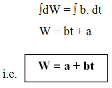
This is the linear growth model.  This is constructed based on the only assumption that ∆W  ∆t.

The Curve:

For linear growth model the curve will be a straight line.

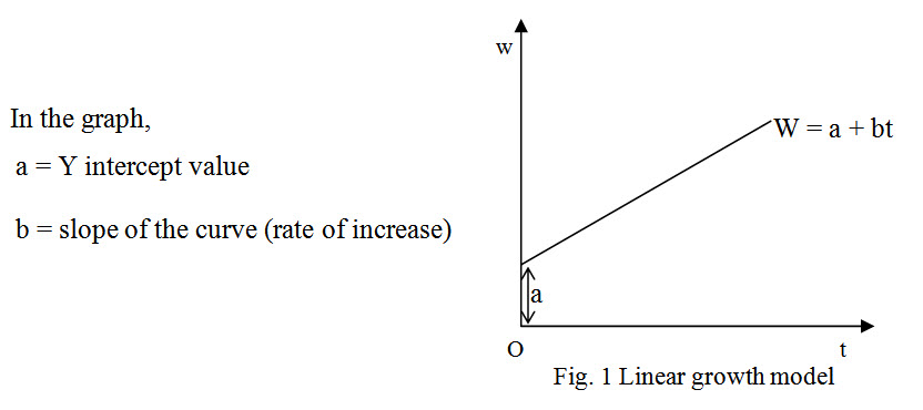
Meaning of the parameters:

In case of linear crop growth model, the parameter ‘a’ indicates the average seed weight and the parameter ‘b’ indicates the crop growth rate (CGR)

Application of the model:

The linear growth model is used only if the curve has the tendency of giving linear trend during the period of investigation or study.  For example, even in response model, for a short period before the optimum point, the curve will be linear.  Similarly, in the crop growth model, suppose we are interested in one particular stage, we can assume that the trend is linear.

We have to plot the observed data in a graph.  If the graph appears to be liner, then we have to estimate the linear model.  For example, in the case of growth model, eventhough entire growth period is sigmoidal, the growth in a growth stage or short period can be assumed to be linear.  Under these circumstances, we can use linear models.  

Estimation of the models:

The linear regression between the dry matter production and time is estimated.

The co-efficients of the linear regression directly give the values of the parameters ‘a’ and ‘b’.

Ex.1. The following observation gives the DMP of IR 20 rice (g plant^-1) at different stages.  Estimate the linear growth model for both the treatments and compare the results.

Time (days)		5	15	25	35	45
DMP (g plant-1)	T1	0.05	0.40	2.97	21.93	162.06
	T2	0.06	0.45	3.42	20.80	160.52

 

Solution:

The linear growth model is estimated.  The estimated model parameters are

Parameter	T1	T2
a	-48.9055	-48.2675
b	3.4555	3.4127
r	0.778	0.776

The estimated linear growth models for the treatments T₁ and T₂ are:

For T₁  :           Ŵ= - 48.9055 + 3.4555 t

For T₂  :           Ŵ= - 48.2675 + 3.4127 t

Exponential Growth Model:

The Model:

Let  W = f (t) be the growth function.

                        Where W = dry matter production (g plant^-1)

                                      t = time (days)

In the linear growth model, the only assumption is that the crop will grow during its growth period (i.e. we make the assumption ΔW  Δt).  But, we know that the growth of any crop in a particular period (say 15^th day) depends on its growth upto that period (growth upto15^th day).  That is, any change in crop growth is also directly proportional to the growth upto the period.  If we include this assumption also, the resulting model is known as exponential growth model.

Assumptions of the model:

In exponential growth model, we have the following two assumptions.

1. Change in growth is proportional to change in time i.e. ∆W   ∆t.

2. Change in growth is also proportional to growth upto that stage i.e. ∆W  W.

Construction of the model:

Combining these two assumptions,

            ∆W  W. ∆t

         ∆W = b. W. ∆t            where b = proportionality constant

            ∆W/ ∆t = b.W

Making  Δt  as the smallest possible value i.e. ∆t → 0

            Lt  ∆t → 0  ∆W/ ∆t = b.W

    i.e.   dW/dt = b.W

            dw/W = b. dt

Integrating both sides,

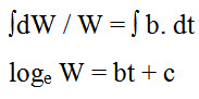
Raising both sides to the power of e,

e^{log W} = e^{bt + c}

W = e^bt. E^c

 W = a e^bt

 

                                               

The Curve:

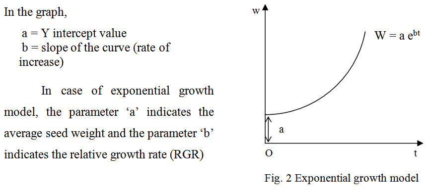
Biological meaning of the parameters:

3. Substitute t=o in the model.  Then we get,

W₀ = a e^{b x 0}

                                          = a e⁰

                                          = a

The parameter ‘a’ gives the growth when t=0. i.e. the average seed weight is given by the parameter ‘a’.

 4. Differentiating the model with respect to t,

                        dW/dt =  a . e^bt . b

                                    = W.b

                                b  = (dW/dt) . (1/W)

i.e.   b = RGR

Application of the model:

As soon as we collect the observation, we should plot the data in a graph.  If the graph is of the type shown in Fig. 2, then we can use exponential growth model.  Moreover, if we know that the crop or situation previously and if the observation collected suits the two assumptions of the model, then we can use the model.  Also, if we are interested only for a period with these two assumptions alone, then also we can decide that the model is exponential growth model. 

Estimation of the model:

W = a e^bt

Taking log on both sides,

log W = log a + bt log e

log W = log a + bt

This is of the form

Y = A + B t

where  Y = log W

A = log a         or         a = e^A

B = b               or         b = B

Ex. 2. The following observation gives the DMP of IR 20 paddy during its growth period.  By estimating  exponential growth model estimate RGR and growth rate on 30^th day.

Time (days)	5	15	25	35	45
DMP (g plant-1)	0.05	0.40	2.97	21.93	162.03

The average seed weight is found to be 0.02 g.

Solution:

The exponential growth model is estimated by estimating the liner regression between  log W and t.  The estimated model parameters are

a = 0.0188                               b = 0.2017                   (r = 0.999)

The estimated model is

Ŵ= 0.0188 e^{0.2017 t}