LESSON 3. Logistic Growth Model

Logistic Growth Model:

The Model:

Let W = f (t) be the growth function.

Where W = dry matter production (g plant^-1)

t = time (days)

In exponential growth model we have assumed on the growth system that the changes in growth is directly proportional to

Changes in time and

Growth upto the period

If we consider the complete growth period of any species, these two assumptions will not be sufficient since these two assumptions are true only upto a particular period and there is a restriction. That is, this will be true only upto the maximum growth. If we include this assumption also i.e. the changes in growth is also directly proportional to W_m-W, where Wm is the maximum possible growth, then the resulting model is known as logistic growth model.

Assumptions of the model:

The assumptions of the logistic growth model are

Change in growth is proportional to change in time i.e. ΔW Δt.
Change in growth is also proportional to growth upto that stage i.e. ΔW W.
Also, the crop will grow upto the maximum growth only i.e. ΔW W_m-W.

Construction of the model:

Combining the three assumptions of the model we get

∆W ∆t. W. (W_m-W)

∆W = k. ∆t.W.(W_m-W) where k = proportionality constant

∆W/ ∆t = k.W.( W_m-W)

Making ∆t as the smallest possible value i.e. ∆t → 0

Lt ∆t → 0 ∆W/ ∆t = k.W.( W_m-W)

i.e. dW/dt = k.W.( W_m-W)

dw/(W ( W_m-W)) = k. dt

Integrating both sides,

M 8 L 3 eq.2

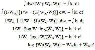
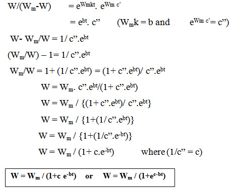
Raising both sides to the power of e

M 8 L 3 eq.3

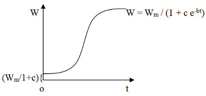
The Curve:

The curve will be of sigmoidal shape.

M 8 L 3 eq.4

Meaning of the parameters:

1. When t = 0, W = W₀ = Seed weight

e^-bt = e⁰ = 1

W0 = Wm / (1+c)

1+c = Wm / W0

c= (Wm / W0) – 1

c is the ratio of maximum possible growth to the initial seed weight minus 1.

2. When there is no restriction i.e. t = µ

e^-bt = e^µ = 0

W = W_m / 1+0 = W_m

i.e. when there is no restriction, W= W_m

Application of the model:

Logistic growth model is used when the complete growth period is considered.

Estimation of Growth Rate:

W = W_m / (1+ c.e^-bt)

dW/dt = {(1+ c.e^-bt) . 0 - W_m (c.e^-bt) (-b)}/ {1+ c .e^-bt}²

= {W_m c.b.e^-bt}/ {1+ c .e^-bt}²

Estimation of the model:

W = W_m / (1+ c.e^-bt)

W / W_m = 1+ c.e^-bt

(W/W_m)-1 = c.e^-bt

Taking log on both sides,

log {(W/ W_m)-1} = log c + log e^-bt

= log c – bt

This is of the form

Y = A+ Bx

Where Y = log {(W/ W_m)-1} x = t

A = log c or c = e^A

B = -b or b = -B

Ex.3. Estimate logistic growth model and obtain its growth rate on 50^th day for the following observation in TMV 7 groundnut.

Time (days)	15	25	45	60	80	95	105	110
DMP (g pl^-1)	3.25	5.30	13.50	25.32	36.96	42.44	45.70	47.45

It is observed that the maximum growth in the replicated plot is 48.5 g pl^-1.

Solution:

The linear regression between log {(W/ W_m)-1} and t is estimated. The estimated co-efficients are

A = 3.7200 B = - 0.0633 (r = -0.993)

The estimated model parameters are

c = e^A = e^3.7200 = 41.2631

b = -B = 0.0633

The estimated logistic growth model is

Ŵ= 48.5 / {1 + 41.2631 e^-0.0633t}

Last modified: Thursday, 27 March 2014, 9:12 AM

System Engineering

LESSON 3. Logistic Growth Model