Site pages
Current course
Participants
General
MODULE 1. Systems concept
MODULE 2. Requirements for linear programming prob...
MODULE 3. Mathematical formulation of Linear progr...
MODULE 5. Simplex method, degeneracy and duality i...
MODULE 6. Artificial Variable techniques- Big M Me...
MODULE 7.
MODULE 8.
MODULE 9. Cost analysis
MODULE 10. Transporatation problems
LESSON 4. Richard’s Growth Model
The model:
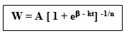
Richard had developed a logistic growth model for predicting the crop growth. The general form of Richard’s growth models is
W = A [ 1 ± e![]() (t)]-1/n
(t)]-1/n
where A = maximum growth
![]() (t) = growth polynomial in t
(t) = growth polynomial in t
If n is positive, we will choose 1 + e![]() (t) and if n is negative we will choose 1 – e
(t) and if n is negative we will choose 1 – e![]() (t). For crop growth, we choose the sign of ‘n’ as positive and polynomial
(t). For crop growth, we choose the sign of ‘n’ as positive and polynomial ![]() (t) = β - kt. Therefore, Richard’s growth model is of the form
(t) = β - kt. Therefore, Richard’s growth model is of the form
where A = maximum growth
β, k and n = model parameters
If n =1, Richard’s growth model reduces to logistic growth model. Normally for annual crops, the value of ‘n’ will be in and around one. The mean relative growth rate is given by the formula R = k / (n+1)
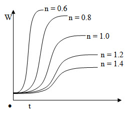
The Richard’s growth curve:
Richard’s growth model follows sigmoidal curve. If the value of n is 1, then the curve will be almost at 45 degrees to X axis.
If the value of n is more than 1, the curve tends to fall down wards and if the value of n is less than 1, the curve becomes more upright.
Estimation of the model:
W = A [1 + eβ - kt]-1/n
W/A = [1 + eβ - kt]-1/n
Raising to the power ‘-n’ on both sides,
(W/A)-n = 1 + eβ - kt
(A/W)n = 1 + eβ - kt
(A/W)n – 1 = eβ - kt
Taking log on both sides,
log{(A/W)n –1} = log eβ – kt
= β – kt = β + (- k) t
This is of the form Y = A + B x
Where Y = log {(A/W)n –1} x = t
A = β or β = A
B = -k or k = -B
We get the values of b and k by estimation. To estimate the above form, we have to assume the value of n. By estimating the value of R2 and χ2, we have to choose the most accurate value of n. We should choose ‘n’ such that χ2 value is minimum.
Ex.4. The following data gives the growth of LRA cotton grown during 1997 at TNAU in two nutrient treatments. Estimate Richards growth models for both the treatments and test their validity.
|
Time |
20 |
40 |
60 |
80 |
100 |
120 |
140 |
160 |
|
T1(g pl-1) |
0.256 |
0.921 |
2.640 |
7.691 |
38.821 |
75.943 |
118.464 |
158.840 |
|
T2(g pl-1) |
0.360 |
0.943 |
2.060 |
7.621 |
32.453 |
65.673 |
105.460 |
140.480 |
The maximum growth in T1 is 160 g pl-1 and in T2 145 g pl-1. Choose the value of n for T1 as 1.26 and T2 as 1.14.
Solution:
The linear regression between log {(A/W)n –1} and t is estimated and the estimated co-efficients are
For T1 A = 10.144 B = - 0.0847 (r = 0.987)
For T2 A = 8.6869 B = - 0.0708 (r = 0.994)
The estimated model parameters are
For T1 β = 10.144 k = 0.0847
For T2 β = 8.6869 k = 0.0708
The estimated growth models are
For T1 Ŵ= 160 [1 + e10.144 –0.0847 t]-0.7937
For T2 Ŵ= 145 [1 + e8.6869 – 0.0708 t]-0.8772
Validity of the models
Time(Days) |
T1 |
T2 |
||
|
W1 |
Ŵ1 |
W2 |
Ŵ2 |
|
|
20 |
0.256 |
0.196 |
0.360 |
0.246 |
|
40 |
0.921 |
0.750 |
0.943 |
0.851 |
|
60 |
2.640 |
2.865 |
2.060 |
2.923 |
|
80 |
7.691 |
10.752 |
7.621 |
9.810 |
|
100 |
38.821 |
36.971 |
32.453 |
30.170 |
|
120 |
75.943 |
93.030 |
65.673 |
72.312 |
|
140 |
118.464 |
140.290 |
105.460 |
115.680 |
|
160 |
158.840 |
155.917 |
140.480 |
136.501 |
|
χ2 |
7.628 |
2.607 |
||
Since the calculated χ2 values are lower than the table χ2 value, there is no significant differences between the predicted and observed values. i.e. the models predict the crop growth satisfactorily and hence can be accepted.
Gompertz’z Growth Model:
The model :
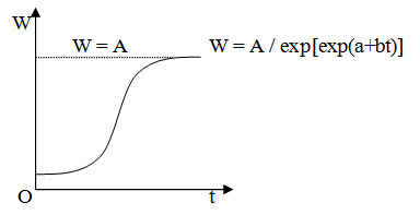
Gompertz’s growth model is of the form
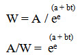
W = A / exp[exp(a+bt)]
Where A = maximum growth
a and b = model parameters
The curve:
The curve is sigmoidal in shape
Estimation of growth rate:
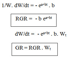
In Gompertz’s growth model, the relative growth (RGR) and growth rate (GR) can be estimated as below
(a + bt)
W = A / ee
Taking log on both sides,
(a + bt)
Log W = log A –log ee
= log A – ea+bt
Differentiating with respect to t,
Estimation of the model:
Taking log on both sides,
log (A/W) = ea+bt
Taking log again
log [log (A/W)] = a + bt
This is of the form Y = a + bx
where Y = log [log (A/W)] and x = t
The co-efficients directly give the values of the parameters ‘a’ and ‘b’.
Ex.5. The following observation gives maize growth in two treatments. T1 is herbicide spray and T2 is hand weeding. Using Gompertz’s growth model, discuss which of the weed management practice is better, by estimating the RGR and GR on 20,40 and 60th day.
|
Time |
10 |
20 |
30 |
40 |
50 |
60 |
80 |
100 |
120 |
|
T1 |
1.74 |
2.69 |
6.40 |
25.81 |
82.34 |
112.39 |
134.26 |
162.10 |
199.88 |
|
T2 |
1.79 |
2.76 |
6.31 |
24.97 |
73.98 |
113.43 |
142.12 |
160.41 |
199.85 |
The maximum growth was found to be 200 g plant-1 for both treatments.
Solution:
The linearity between log [log (A/W)] and t were estimated. The estimated model parameters are
For T1 a = 3.1440 b = - 0.066 (r = -0.0887)
For T2 a = 3.1073 b = -0.0654 (r = -0.893).
The estimated models are
For T1 Ŵ1 = 200 / exp[exp(3.144 – 0.066t)]
For T2 Ŵ2 = 200/ exp[exp(3.1073 – 0.0654t)]
Validity of the models
Time(Days) |
T1 |
T2 |
||
|
W1 |
Ŵ1 |
W2 |
Ŵ2 |
|
|
10 |
1.74 |
0.0012 |
1.79 |
0.0018 |
|
20 |
2.69 |
0.4073 |
2.76 |
0.4737 |
|
30 |
6.40 |
8.1303 |
6.31 |
8.6273 |
|
40 |
25.81 |
38.2058 |
24.97 |
39.0123 |
|
50 |
82.34 |
85.0091 |
73.98 |
85.4966 |
|
60 |
112.39 |
128.5246 |
113.43 |
128.5644 |
|
80 |
134.26 |
177.7167 |
142.12 |
177.4783 |
|
100 |
162.10 |
193.7874 |
160.41 |
193.6433 |
|
120 |
199.88 |
198.3212 |
199.85 |
198.2611 |
|
χ2 |
2554.63 |
1809.28 |
||
The estimated RGR and GR at 20th, 40th and 60th days are
Time(Days) |
T1 |
T2 |
||
|
RGR |
GR |
RGR |
GR |
|
|
20 |
0.409 |
0.167 |
0.395 |
0.187 |
|
40 |
0.109 |
4.164 |
0.107 |
4.174 |
|
60 |
0.029 |
3.727 |
0.029 |
3.728 |
Inference
Since the calculated χ2 values are greater than the table χ2 value at 8 d.f., there exists significant difference between the predicted and observed values. i.e. the model do not estimate the crop growth correctly. Therefore, the models can not be used for this data.
The following can be inferred from the RGR and GR values,
Herbicide spray (T1) registered high RGR than Hand weeding (T2) at 20. 40 and 60 days. Therefore T1 is better than T2.
Hand weeding (T2) registered higher GR at 20 and 40 days than herbicide spray (T2) probably due to better control of weeds. However at 60 days, there is no difference in GR between treatments.
Gauss Growth Model:
The Model:
The Gauss growth model is of the form
W = A [1 – exp(a+bt2)]
Where A = maximum possible growth
a and b = model parameters
Estimation of growth rate:
The growth rate of Gauss curve is of the form,
GR = dW/dt = A . [- exp (a+bt2)] . 2bt
= - 2 Abt . exp(a+bt2)
Estimation of the model:
W = A [1 – exp(a+bt2)]
W/A = 1 – exp(a+bt2)
1-W/A = exp(a+bt2)
Taking log on both sides,
Log (1-W/A) = a + bt2
i.e. Y = a + b X
where Y = log (1-W/A) and X = t2
Ex.6. The following observation gives the growth of maize in two seasons under the same treatment. Test whether there is a change in growth rate between the seasons in maize growth or test whether the season has any influence on maize growth.
|
Time |
10 |
20 |
30 |
40 |
50 |
60 |
80 |
100 |
120 |
|
W1 |
1.23 |
2.09 |
5.90 |
24.80 |
81.46 |
110.23 |
132.46 |
463.62 |
201.46 |
|
W2 |
1.41 |
2.01 |
5.89 |
22.32 |
74.39 |
101.46 |
124.83 |
148.56 |
182.32 |
The maximum dry weight recorded was 202 g plant-1.
Solution:
The linearity between log (1-W/A) and t2 was estimated. The estimated model parameters are
For T1 a = 0.431 b = - 0.00035 (r = -0.913)
For T2 a = 0.0368 b = - 0.00016 (r = -0.989)
The estimated Gauss growth models are
Season 1 Ŵ1 = 202 [1 – exp(0.431 – 0.00035 t2)]
Season 2 Ŵ2 = 202 [1 – exp(0.0368 – 0.00016 t2)]
Validity of the models
Time(Days) |
Season 1 |
Season 2 |
||
|
W1 |
Ŵ1 |
W2 |
Ŵ2 |
|
|
10 |
1.23 |
-98.15 |
1.41 |
-4.25 |
|
20 |
2.09 |
-68.23 |
2.01 |
5.42 |
|
30 |
5.90 |
-24.45 |
5.89 |
20.53 |
|
40 |
24.80 |
24.45 |
22.32 |
39.76 |
|
50 |
81.46 |
72.42 |
74.39 |
61.52 |
|
60 |
110.23 |
113.83 |
101.46 |
84.19 |
|
80 |
132.46 |
168.91 |
124.83 |
126.73 |
|
100 |
163.32 |
192.61 |
148.56 |
159.69 |
|
120 |
201.46 |
199.99 |
182.32 |
181.07 |
The estimated growth rates are
|
Time |
10 |
20 |
30 |
40 |
50 |
60 |
80 |
100 |
120 |
GRW1 |
2.10 |
3.78 |
4.76 |
4.97 |
4.53 |
3.70 |
1.85 |
0.66 |
0.17 |
|
GRW2 |
0.66 |
1.26 |
1.74 |
2.08 |
2.25 |
2.26 |
1.93 |
1.35 |
0.80 |
Inference
The growth rates are higher in season 1 at all stage of growth than in season 2. Therefore, it can be concluded that season has an influence on growth rate of maize. The estimated growth at 10, 20 and 30 days are negative. Since, in biological systems, the growth can not be negative, the models do not estimate the growth properly. Therefore, the models can not be accepted for predicting maize growth.
Last modified: Thursday, 27 March 2014, 7:13 AM