Engineering Physics 3(2+1)

LESSON 3. Adiabatic Demagetization & its properties

 

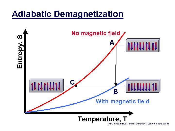
Adiabatic Demagnetization diagram

What are Paramagnetic Materials?

When an outside magnetic field is applied to these materials, a magnetic field that is parallel to the applied field is induced.  The amount of particles that align with the applied field depends on the field strength: if there is higher field strength, more particles are aligned with the field.

The Process of Adiabatic Demagnetization

• First, the sample to be cooled (typically a gas) is allowed to touch a cold reservoir (which has a constant temperature of around 3-4 K, and is often liquid Helium), and a magnetic field is induced in the region of the sample.

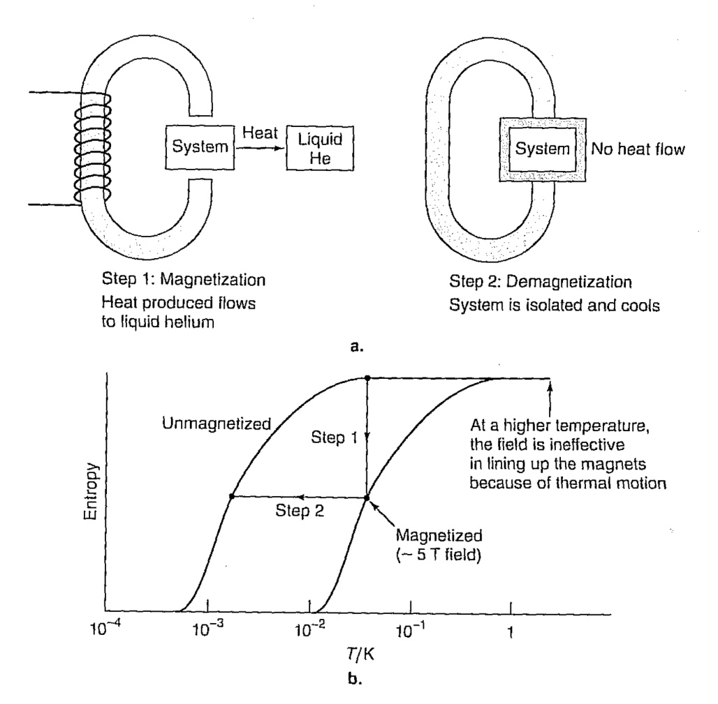
Fig.2(2) Process of adiabatic demagnetization

• Once the sample is in thermal equilibrium with the cold reservoir, the magnetic field strength is increased.  This causes the entropy of the sample to decrease, because the system becomes more ordered as the particles align with the magnetic field.  The temperature of the sample is still the same as that of the cold reservoir at this point.
• Then the sample is isolated from the cold reservoir, and the magnetic field strength is reduced.  The entropy of the sample remains the same, but its temperature drops in reaction to the reduction in the magnetic field strength.  If the sample was already at a fairly low temperature, this temperature decrease can be ten-fold or greater.
• This process can be repeated, permitting the sample to be cooled to very low temperatures.

Limitations of the Process of Adiabatic Demagnetization

If the sample material is an electronic paramagnet, the lowest temperatures that can be attained using these methods are on the order of 1 milliKelvin.

If the sample is a nuclear paramagnet, the lowest achievable temperatures are much lower (because the interactions between the dipoles are much weaker).  

Weiss Molecular Field Theory and Ferromagnetism Or

Weiss theory of Ferromagnetism Or

Mean Field Theory of Ferromagnetism Or

Molecular Theory of Ferromagnetism

It has been observed that the ratio of the magnetic moment to the angular momentum    for the spinning electron is twice for an orbital electron. In case of ferromagnetic materials this ratio is almost same as that for a spinning electron. Hence, the spinning electrons make a major contribution to magnetic properties of ferromagnetic.

According to Weis, the effective field strength  may be regarded as the vector sum of external applied field strength  and the internal molecular field strength B_i

\[{B_e}=B + {B_i}=B + \lambda I\]…… (1)

Consider gram molecule of the substance whose density is  and molecular weight  and   and  being the gram molecular moment and its saturation value respectively then

And

\[{I_s} = {{{\sigma _s}\rho } \over M}\]……….. (3)

Since I  and I_s  refer to the unit volume

\[{I \over {{I_s}}}\] = \[{\sigma\over{{\sigma _s}{\rm{}}}}\]………… (4)

As the domains are assumed to obey the general theory of paramgnetism, then from Langevin’s theory of paramgnetism, we have

\[{I \over {{I_s}}}=L\left( a \right)=\left[{\cot a -{1\over a}}\right]\]…………. (5)

Equating (4) and (5)

\[{I \over {{I_s}}}\] = \[{\sigma\over{{\sigma _s}{\rm{}}}}\]  = \[L\left(a\right)=\left[{\cot a-{1\over a}}\right]\]………….. (6)

Where \[{{\mu {B_e}}\over {KT}}\] = a =  \[{{\mu \left( {B + \lambda I} \right){\rm{}}} \over {KT}}\]…….. (7)

When the external field is zero  B = 0

\[{B_e}=\lambda I={{\lambda \sigma \rho } \over M}\]…………. (8)

 Putting equation (8) in equation (7)

\[{\mu\over{KT}}{{\lambda\sigma\rho}\over M}\] = a = \[{{{\sigma _o}} \over N}\] \[{{\lambda \sigma \rho } \over {MKT}}={{{\sigma _o}} \over N}{{\left( {B + \lambda I} \right){\rm{}}} \over {KT}}\]

Hence

\[{\sigma\over{{\sigma _o}}}={{RMT} \over {\lambda \rho {\sigma _o}^2}}a\]……… (9)

 

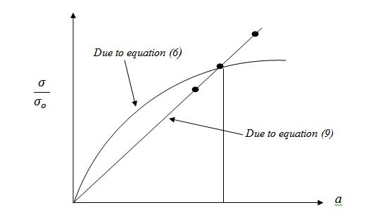
Equation (9) and (7) simultaneously determine the condition for spontaneous magnetization.