Engineering Physics 3(2+1)

LESSON 11. Qualitative Explanation of Zeeman Effect

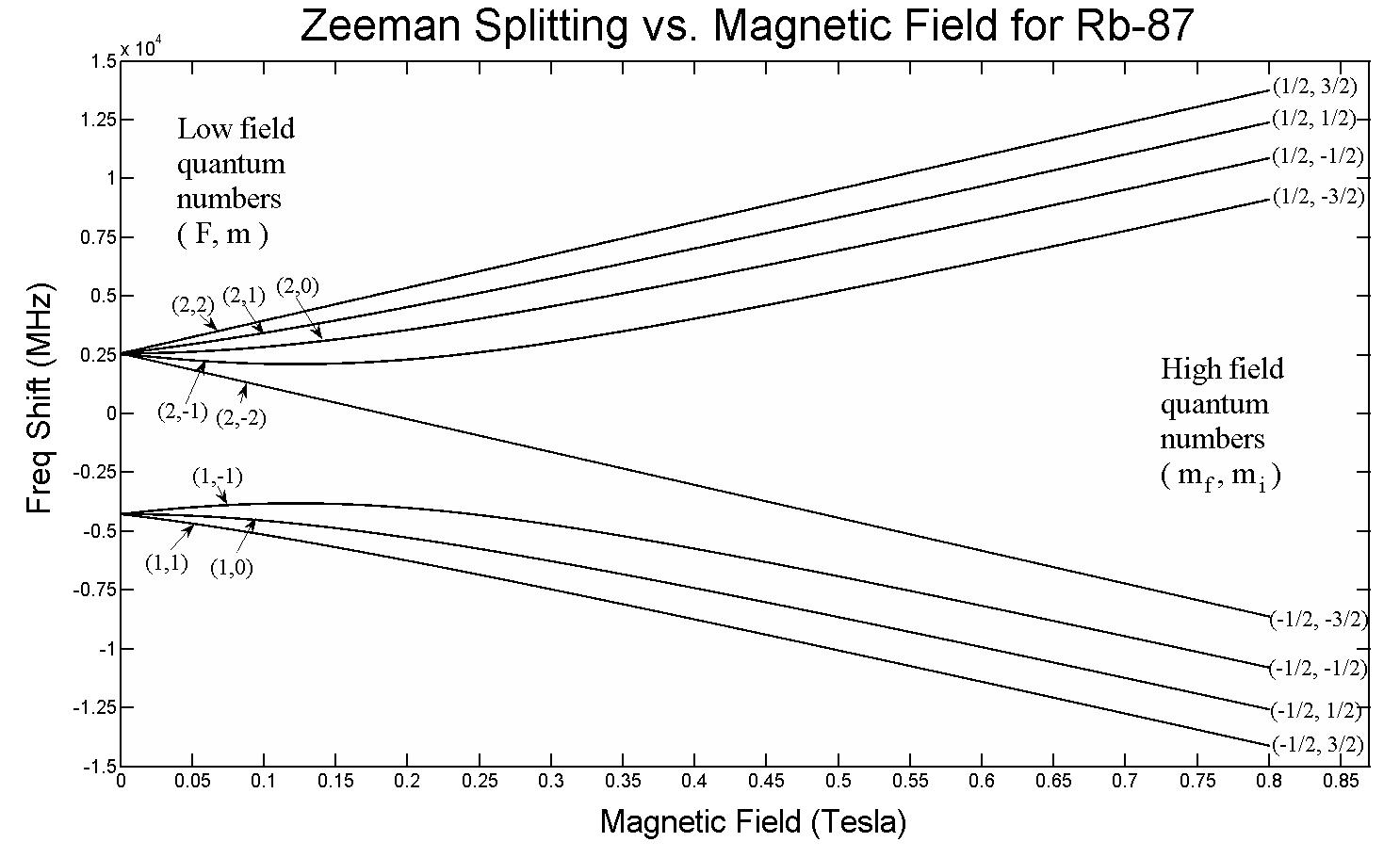
 Fig Zeeman Splitting against Magnetic Field

Also similar to the Stark effect, transitions between different components have, in general, different intensities, with some being entirely forbidden (in the dipole approximation), as governed by the selection rules.

The distance between the Zeeman sub-levels is a function of the magnetic field; this effect can be used to measure the magnetic field

The Zeeman Effect is very important in applications such as nuclear magnetic resonance spectroscopy, electron spin resonance spectroscopy, Magnetic Resonance Imaging (MRI).

It may also be utilized to improve accuracy in atomic absorption spectroscopy. A theory about the magnetic sense of birds assumes that a protein in the retina is changed due to the Zeeman Effect.

When the spectral lines are absorption lines, the effect is called inverse Zeeman Effect.

Theoretical Background

The total Hamiltonian of an atom in a magnetic field is

H = H₀ + V_M ,

where H₀ is the unperturbed Hamiltonian of the atom, and V_M is perturbation due to the magnetic field:

where  is the magnetic moment of the atom. The magnetic moment consists of the electronic and nuclear parts; however, the latter is many orders of magnitude smaller and will be neglected here. Therefore,

where is the Bohr magneton, is the total electronic angular momentum, and g is the Landé g-factor. The operator of the magnetic moment of an electron is a sum of the contributions of the orbital angular momentum  and the spin angular momentum , with each multiplied by the appropriate gyromagnetic ratio:

where g_{l = 1}  and (the latter is called the anomalous gyromagnetic ratio; the deviation of the value from 2 is due to Quantum Electrodynamics effects). In the case of the LS coupling, one can sum over all electrons in the atom:

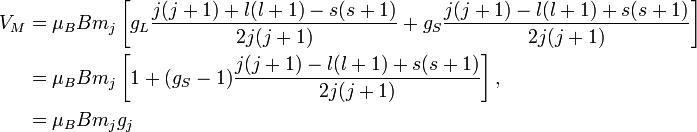
Where   and  are the total orbital momentum and spin of the atom, and averaging is done over a state with a given value of the total angular momentum.

If the interaction term V_M is small (less than the fine structure), it can be treated as a perturbation; this is the Zeeman Effect proper. In the Paschen-Back effect, described below, V_M exceeds the LS coupling significantly (but is still small compared to H₀). In ultra strong magnetic fields, the magnetic-field interaction may exceed H₀, in which case the atom can no longer exist in its normal meaning, and one talks about Landau levels instead. There are, of course, intermediate cases which are more complex than these limit cases.

If the spin-orbit interactions dominate over the effect of the external magnetic field and   are not separately conserved, only the total angular momentum is. The spin and orbital angular momentum vectors can be thought of as processing about the (fixed) total angular momentum vector. The (time-)"averaged" spin vector is then the projection of the spin onto the direction of :

and for the (time-)"averaged" orbital vector:

Thus,

Using  =  - and squaring both sides, we get

and: using =  -  and squaring both sides, we get

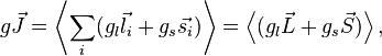
 Combining everything and taking , we obtain the magnetic potential energy of the atom in the applied external magnetic field,

 

where the quantity in square brackets is the Landé g-factor gJ of the atom ( and ) and  ^mj is the z-component of the total angular momentum. For a single electron above filled shells s = 1 and j = 1 ± s, the Landé g-factor can be simplified into:

The Lyman alpha transition in hydrogen in the presence of the spin-orbit interaction involves the transitions

  and

In the presence of an external magnetic field, the weak-field Zeeman effect splits the 1S1/2 and 2P1/2 levels into 2 states each (mj =1/2,-1/2) and the 2P3/2 level into 4 states (mj = 3/2,1/2,-1/2,-3/2).

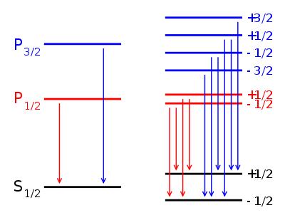
Fig. Zeeman Splits

The Landé g-factors for the three levels are:

g_{J = 2} For (j=1/2, l=0)

g_{J = 2}/3 For (j=1/2, l=1)

g_{J = 4/3}  For (j=3/2, l=1).

Note in particular that the size of the energy splitting is different for the different orbital, because the gJ values are different. On the left, fine structure splitting is depicted. This splitting occurs even in the absence of a magnetic field, as it is due to spin-orbit coupling. Depicted on the right is the additional Zeeman splitting, which occurs in the presence of magnetic fields.