Ground Water,Wells and Pumps 3(2+1)

Lesson 3 Aquifer and Its Properties

We have learned in Lesson 2 that most common aquifer materials are unconsolidated sands and gravels, which occur in alluvial valleys, old stream beds covered by fine deposits (buried valleys), coastal plains, dunes, and glacial deposits. Sandstones are also good aquifer materials. Cavernous limestones with sufficient solution channels, caves, underground streams, and other karst developments can also be high-yielding aquifers. Basalts, lavas, and other materials of volcanic origin can make excellent aquifers if they are sufficiently porous or fractured and if the vesicles are interconnected (in case of lava). However, other sedimentary rocks such as shales, solid limestones, etc. generally don’t serve as good aquifers. Small water yields may be possible where these rocks are highly fractured. The same is true for granite, gneiss, and other crystalline or metamorphic rocks.

 

3.2 Types of Aquifers

Aquifer can be basically classified into three types: (i) unconfined aquifer, (ii) confined aquifer, and (iii) leaky aquifer. Sometimes, fourth type of the aquifer is known as ‘perched aquifer’, but it is not the focus of any groundwater exploration. Fig. 3.1 illustrates the types of aquifers available below the ground.

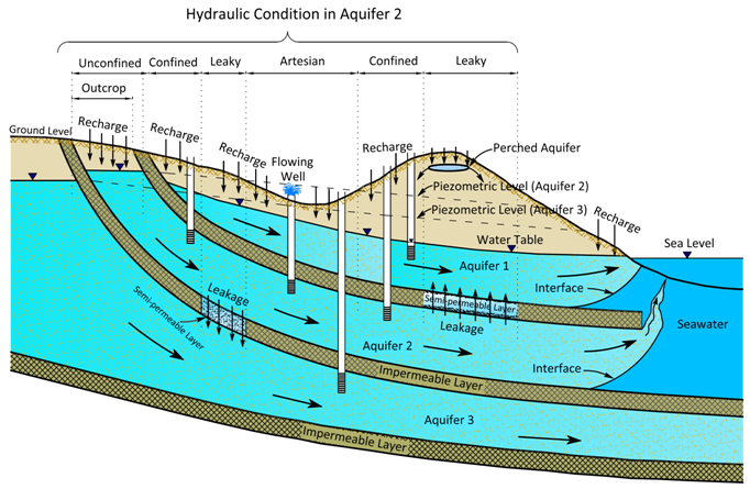
Fig. 3.1. Types of aquifers for groundwater development.

(Source: Bear, 1979)

 

3.2.1 Unconfined Aquifers

Aquifers which are bounded by a free surface (known as ‘water table’) at the upper boundary and a confining layer at the lower boundary are called unconfined aquifers (Aquifer 1 in Fig. 3.1). At the water table, water is at the atmospheric pressure, and hence unconfined aquifers are also called ‘water-table aquifers’ or ‘phreatic aquifers’.

 

Unconfined aquifers receive recharge directly from the overlying surface through rainfall infiltration or percolation from surface water bodies. They usually exhibit a shallow water level. A typical indicator of an unconfined aquifer is that the water level in a well tapping this aquifer is equal to the water table position at that location of the aquifer. In other words, water level doesn’t rise above the water table.

 

3.2.2 Confined Aquifers  

Aquifers which are bounded both above and below by impervious or semi-pervious layers are called confined aquifers and the water present in these aquifers are under pressure (Aquifers 2 and 3 in Fig. 3.1). Confined aquifers are sometimes also called ‘pressure aquifers’ or ‘artesian aquifers’; the latter term is gradually becoming obsolete. Since the water present in a confined aquifer is at a pressure greater than the atmospheric pressure, the water level in a borewell penetrating a confined aquifer will always rise above the top confining layer of the aquifer. The term ‘piezometric level’ is used to denote this water level. Thus, ‘Piezometric level’ is an imaginary position to which the water level will rise in a borewell tapping a confined aquifer. Piezometric level in two dimensions is called ‘piezometric surface’.

 

Unlike unconfined aquifers, confined aquifers don’t receive significant amounts of recharge from the overlying surface. The groundwater within a confined aquifer is under a pressure equal to the sum of the weight of the atmosphere and the overburden. As mentioned above, the groundwater level in a well penetrating a confined aquifer is usually above the upper boundary of the confined aquifer. However, there may be cases where the piezometric level of a confined aquifer is above the ground surface. The well tapping such a confined aquifer yields water like a spring, and hence it is called a ‘flowing well’ and such a confined aquifer is known as an ‘artesian aquifer’. Note that the word ‘artesian’ comes from the name of a place in France where flowing wells were seen for the first time in the world. Hence, this word is now widely understood to refer only to the hydraulic condition in a confined aquifer due to which flowing wells exist (i.e., groundwater flows naturally beyond the ground surface). Unfortunately, some books on groundwater still use the term ‘artesian aquifer’ synonymous with ‘confined aquifer’.

 

Moreover, most confined aquifers are unconfined at their exposed edges in the upstream portion of the aquifer, which is called ‘outcrop’ (Fig. 3.1). They receive significant recharge through the outcrop by direct rainfall infiltration into this unconfined portion. Confined aquifers also receive recharge through their upper and lower leaky confining layers under natural conditions or when pressure changes are artificially induced by pumping or injection. Groundwater flux to and from an aquifer through a confining layer is termed ‘leakage’ (Fig. 3.1) and the confining layer is called a ‘leaky confining layer’ or ‘aquitard’.

 

3.2.3 Leaky Aquifers

If an aquifer (confined aquifer or unconfined aquifer) loses or gains water through adjacent semi-permeable layers, it is called a ‘leaky aquifer’ (Fig. 3.1). Therefore, the terms ‘leaky confined aquifer’ and ‘leaky unconfined aquifer’ are widely used depending on whether the leaky aquifer is confined or unconfined.  However, the case of ‘leaky confined aquifer’ has been mostly dealt with by the groundwater experts. This is why, the term ‘semi-confined aquifer’ is sometimes used to denote a ‘leaky aquifer’. The term ‘nonleaky’ is also used to describe the status of a confined or unconfined aquifer, such as ‘nonleaky unconfined aquifers’ and ‘nonleaky confined aquifers’. In reality, ideal confined aquifers or ideal unconfined aquifers occur less frequently than do leaky aquifers. 

 

3.2.4 Perched Aquifers

A perched aquifer is a special type of an unconfined aquifer, in which water exists under water-table conditions. Therefore, the upper boundary of this aquifer is called ‘perched water table’ (Fig. 3.1). Perched aquifer always exists in the vadose zone above an unconfined aquifer or a confined aquifer when a low-permeability layer impedes the downward movement of water above it. Perched aquifers have generally very limited areal extent and they may not have sufficient storage to support significant well production. Therefore, perched aquifers are not the target of a groundwater exploration. However, perched aquifers can support shallow dug wells, thereby can provide water supply to a small community for a limited time period.

 

It should be noted that hydraulically single aquifers seldom exist in nature. An aquifer is generally part of a system of two or more aquifers, which is more complex. Aquifer thickness, hydraulic head, Darcy velocity, seepage velocity, hydraulic conductivity, transmissivity, intrinsic permeability, storage coefficient (specific storage), specific yield, and specific retention are the important hydraulic and hydrogeologic parameters which are used to characterize an aquifer system. Some of these parameters are discussed in the subsequent section, while others will be discussed in Lesson 4. 

 

3.3 Properties of Aquifers

The hydrogeologic factors which govern the storage and fluid-transmitting characteristics of an aquifer system are called ‘aquifer properties’ or ‘aquifer parameters’. Storage-related aquifer properties (or storage parameters) are: porosity, effective porosity, specific retention, specific yield, storage coefficient, and specific storage. On the other hand, fluid-transmission-related aquifer properties (or yield parameters) are: intrinsic permeability, hydraulic conductivity, and transmissivity. These properties are defined below.

 

3.3.1 Porosity

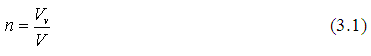
‘Porosity’ (n) of a porous medium (soil or subsurface formation) is defined as the ratio of the volume of voids (V_v) in a porous medium to the total volume of the porous medium (V). That is,

 

                                                        

 

Porosity is a dimensionless parameter and is computed as n = (1- r_b/r_p), where r_b = bulk density of the soil/subsurface formation, and r_p = particle density of the soil/subsurface formation.

 

In general, rocks (consolidated subsurface formations) have lower porosities than soils or unconsolidated subsurface formations. Gravels, sands and silts, which are made up of angular and rounded particles, have lower porosities than the soil rich in platy clay minerals. Also, poorly-sorted deposits/subsurface formations have lower porosities than well-sorted deposits/subsurface formations.

 

3.3.2 Effective Porosity

Because of the presence of isolated (not interconnected) pores, dead-end pores, micropores (i.e., extremely small-size pores), and adhesion forces in a porous medium, only a very small fraction of the total porosity is effective (i.e., permeable). ‘Effective Porosity’ is defined as the portion of void space in a porous material through which fluid (liquid or gas) can flow. In other words, it is the fraction of total porosity which is available for fluid flow. It is also called ‘kinematic porosity’.

 

Like the definition of porosity (total porosity) of a porous medium, effective porosity (n_e) can be defined as follows:

 

         

Note that the definition of effective porosity is linked to the concept of fluid (water or gas) circulation and not to the percentage of the volume occupied by a fluid.

 

3.3.3 Specific Retention

‘Specific Retention’ (S_r) of a soil or aquifer material is defined as the ratio of the volume of water retained after saturation against gravity to its own volume. That is,

 

                                                

 

Where, V_r = volume of retained water, and V = total volume of the soil or aquifer material.

 

It should be noted that S_r increases with decreasing grain size. For example, clay may have a porosity of 50% with a specific retention of 48%. Moreover, the terms ‘field capacity’ and ‘retained water’ refer to the same water content, but differ by the zone in which they occur; the former occurs in the unsaturated zone and the latter in the zone of saturation.

 

3.3.4 Specific Yield

‘Specific Yield’ (S_y) or ‘Drainable Porosity’ of a soil or aquifer material is defined as the ratio of the volume of water that, after saturation, can be drained by gravity to its own volume. That is,

 

                                               

                                               

Where, V_d = volume of water drained by gravity (i.e., drainable volume), and V = total volume of the porous medium (soil or aquifer material).

 

As the volume of water drained (V_d ) and the volume of water retained (V_r) constitute the total water volume in a saturated porous material, the sum of the two is equal to the total porosity (n) of a porous material. That is, 

n = S_y + S_r                                              (3.5a)

                                     

Or,                                           S_y = n - S_r                                               (3.5b)

 

The above basic definition of specific yield is very common in Vadose Zone Hydrology and Groundwater Hydrology and is applied when the specific yield is determined in the laboratory. However, if the specific yield is determined in the field, it is defined as the volume of water released from or taken into storage per unit area of an unconfined aquifer per unit change in water table position. This definition is widely used to estimate seasonal/annual groundwater storage in an area or a basin due to rise in the water table during recharge period as well as to estimate groundwater withdrawal/discharge from an area due to lowering of the water table during the period of groundwater pumping or recession.       

 

Specific yield is a dimensionless parameter of the aquifer. The values of specific yield or drainable porosity depend on the grain size, shape and distribution of pores, compaction of the subsurface formation, and duration of drainage. It should be noted that fine-grained materials yield little water, whereas coarse-grained materials permit a considerable release of water, and hence serve as aquifers. Further, the value of S_y decreases with depth due to compaction. The values of S_y generally range from about 0.01 to 0.30 (Freeze and Cherry, 1979) depending on the type of porous materials present in the saturated zone/aquifer or vadose zone. Table 3.1 shows the typical values of porosity and specific yield (effective porosity) for selected unconsolidated and consolidated formations.

 

Table 3.1. Typical values of porosity and specific yield for different geological materials (Brassington, 1998)

Sl. No.	Type of Geological Material	Porosity (%)	Specific Yield (%)
1	Coarse Gravel	28	23
2	Medium Gravel	32	24
3	Fine Gravel	34	25
4	Coarse Sand	39	27
5	Medium Sand	39	28
6	Fine Sand	43	23
7	Silt	46	8
8	Clay	42	3
9	Fine-grained Sandstone	33	21
10	Medium-grained Sandstone	37	27
11	Limestone	30	14
12	Dune Sand	45	38
13	Loess	49	18
14	Peat	92	44
15	Schist	38	26
16	Siltstone	35	12
17	Till (mainly Sand)	31	16
18	Till (mainly Silt)	34	6
19	Tuff	41	21

 

 3.3.5 Storage Coefficient and Specific Storage

‘Storage Coefficient’ or ‘Storativity’ (S) of an aquifer is defined as the volume of water released from or taken into storage per unit area of an aquifer per unit change in hydraulic head. Here, the hydraulic head denotes ‘piezometric level’ for confined aquifers and ‘water table’ for unconfined aquifers. Figure 3.2 illustrates the concept of storage coefficient (storativity). Thus, the term ‘storage coefficient’ or ‘storativity’ applies to both confined and unconfined aquifers. 

Storage coefficient is a dimensionless aquifer parameter. Mathematically, it is expressed as follows:

S = S_s × b                                                  (3.6)

 

Where S_s = specific storage of the aquifer material, and b = thickness of the aquifer.

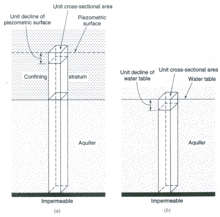
Fig. 3.2. Schematic representation of storage coefficient for: (a) Confined aquifers; (b) Unconfined aquifers. (Source: Todd, 1980)

 

The ‘Specific Storage’ (S_s) of an aquifer is defined as the volume of water released from or taken into storage per unit volume of an aquifer per unit change in hydraulic head. The specific storage has the dimension of [L^-1]. It is mathematically expressed as follows:

 

                                                                (3.7)

 

Where, ρ_w = density of water; α = compressibility of the aquifer material (a is equal to , wherein E_s is bulk modulus of elasticity of aquifer skeleton); β = compressibility of water (β is equal to 1/K_w, wherein K_w is bulk modulus of elasticity of water); n = porosity of the aquifer material; and γ_w = unit weight of water. Thus, the specific storage is a more fundamental aquifer parameter, which depends on the type of aquifer material, water present in the aquifer, and the overburden stress.   

 

The value of K_w (bulk modulus of elasticity of water) is 2.1X10⁹ N/m², whereas the values of E_s (bulk modulus of elasticity of aquifer skeleton) for some geological materials are given in Table 3.2 (Raghunath, 2007).

 

Table 3.2. Values of E_s for selected geological materials (Raghunath, 2007)

Sl. No.	Geological Material	Value of Es (N/m2 ´ 105)
1	Plastic clay	5-40
2	Stiff clay	40-80
3	Medium-hard clay	80-150
4	Loose sand	100-200
5	Dense sand	500-800
6	Dense sandy gravel	1,000-2,000
7	Fissured or Jointed Rock	1,500-30,000
8	Sound Rock	>30,000

 

If we substitute Eqn. (3.7) in Eqn. (3.6), the expanded form of the equation for storage coefficient (storativity) would be: 

                                             (3.8) 

It is obvious from Eqn. (3.8) that besides the aquifer compressibility (α) and water compressibility (β), the storage coefficient (S) of an aquifer is a function of aquifer thickness (i.e., aquifer geometry) which is a location-specific quantity, and hence it varies from one location to another over a basin or sub-basin. Note that the expression of storage coefficient [Eqn. (3.8)] consists of two parts: (i) the amount of water released from an aquifer or taken into aquifer storage due to the compressibility of the aquifer material/skeleton (S_c), which is expressed as, and (ii) the amount of water released from an aquifer or taken into aquifer storage due to the compressibility of water (S_w), which is expressed as.

 

It is worth mentioning that the phenomena of aquifer compression and water expansion due to drop in the groundwater level also occur in unconfined aquifers. However, their contribution to the volume of water released by an unconfined aquifer is negligible in most cases as compared to the volume of water derived from the gravity drainage of pores. Therefore, for practical purposes, the storage coefficient (S) is equal to the specific yield (S_y) for unconfined aquifers and the concept of specific storage is almost exclusively used for the analysis of confined aquifers

 

The values of storage coefficient (S) of confined aquifers are relatively small and they often range from 0.005 to 0.00005 (Freeze and Cherry, 1979). It indicates that large pressure changes over extensive areas are required to produce substantial water yields from a confined aquifer. Considering the range of values of specific yield (S_y) mentioned above, it is clear that the specific yield of unconfined aquifers is considerably higher than the storage coefficient of confined aquifers.

 

3.3.6 Intrinsic Permeability

‘Intrinsic permeability’ or ‘permeability’ of porous media (soils or subsurface formations) is defined as their ability to transmit a fluid (liquid or gas) through them. It is a property of the medium only and is independent of the fluid properties. Intrinsic permeability (k) is mathematically expressed as follows:

 

k = Cd²                                                      (3.9)

 

Where, C = dimensionless proportionality constant commonly known as ‘shape factor’ (accounting for the shape of pore space which is a function of mean grain diameter, sphericity and roundness of grains, distribution of grain sizes, and nature of their packing), and d = diameter of the pore space (also known as ‘characteristic grain diameter’ or ‘characteristic length’).

 

The dimension of k is [L²] and its SI unit is m². Because of very small values of k, it is also expressed in square micrometers [(mm)²], i.e., 10^-12 m². However, in the petroleum industry, the value of k is measured in a unit termed ‘darcy’, which is defined as (Todd, 1980):

 

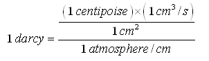
Note that 1 darcy = 0.987 (mm) ² = 0.987×10^-8 cm².

 

3.4 Water Yielding Mechanisms of Aquifers

Unconfined aquifers yield water to wells or other water collection facilities due to actual drainage (dewatering) of pores. Air replaces the water initially present in the dewatered zone as the water table drops from a higher elevation to a lower elevation. Thus, the water released from an unconfined aquifer is mainly derived from the dewatering of pores (voids). Therefore, the storage coefficient (S) for an unconfined aquifer corresponds to its specific yield (S_y).

Note that if the water table lowers at a rapid rate due to large pumping rate, the drainage of pores may not take place sufficiently fast to deliver the full specific yield. In this case, continued drainage of pores will occur for some time even if the water table has already receded to lower levels. Thus, the specific yield of an aquifer is dependent on the rate of fall of water table, and varies with time and distance from a pumping well.

On the other hand, confined aquifers remain completely saturated, and hence it does not release water due to drainage of pores. In confined aquifers, water is basically released from or taken into storage as a result of changes in pore volume due to aquifer compressibility and water compressibility (changes in water density associated with a change in pore-water pressure). Thus, confined aquifer releases water due to the compression of aquifer material and the expansion of water (decrease in water density owing to the decrease in pore-water pressure). Therefore, the capacity of confined aquifers to release water from storage is remarkably different from that of the unconfined aquifers. In other words, the amount of water yielded by these mechanisms per unit drop in piezometric level is considerably less than that yielded by the drainage of pores per unit drop in water table. Besides these two primary water-yielding mechanisms, the confined aquifers also yield water by other two mechanisms (Bouwer, 1978): (i) leakage from adjoining aquifers through aquitards (e.g., an overlying unconfined aquifer or an underlying confined aquifer), and (ii) direct draining of pores at the outcrop of a confined aquifer or if the confined aquifer hydraulically becomes an unconfined aquifer when the piezometric level in a confined aquifer drops to or below the bottom of its top confining layer.

 

3.5 Example Problems

3.5.1 Example Problem 1

In an unconfined aquifer extending over 4 km², the water table was initially at 26 m below the ground surface. Sometime after an irrigation of 20 cm (full irrigation), the water table rises to a depth of 25.5 m below the ground surface. Afterward 1.5 ´ 10⁶ m³ of groundwater was withdrawn from this aquifer, which lowered the water table to 27.5 m below the ground surface. Determine: (i) specific yield of the aquifer, and (ii) soil moisture deficit (SMD) before irrigation.

Solution:

(i)  Volume of groundwater withdrawn from the unconfined aquifer =          Area of the aquifer ´ Drop in the water table ´ Specific yield

 

Substituting the values, we have,

 

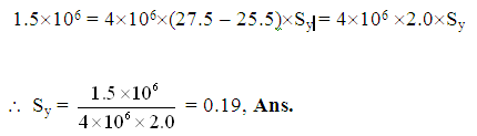
(ii) Volume of water recharged due to irrigation (V_R) = Area of the aquifer influenced by irrigation ´ Rise in the water table ´ S_y 

Let us consider the aquifer area influenced by irrigation to be 140 m², then the volume of water recharged (V_R) will be: 

V_R = 140´X(26.0-25.5)´0.19 = 13.3 m³ 

Volume of irrigation water (V_I) = 140 × 0.20 = 28.0 m³ 

Now, Soil moisture deficit (SMD) before irrigation = V_I - V_R = 28.0-13.3 = 14.7 m³. 

Or, SMD = = 0.105 m = 10.5 cm, Ans.

 

3.5.2 Example Problem 2

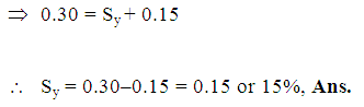
In an area of 200 ha, the water table declines by 3.5 m. If the porosity of the aquifer material is 30% and the specific retention is 15%, determine: (i) specific yield of the aquifer, and (ii) change in groundwater storage.

 

Solution:

(i)  We know, Porosity = Specific yield (S_y) + Specific retention (S_r)

 

(ii) Change in groundwater storage = Area of the aquifer ´ Drop in the water table ´ Specific yield

                                                      = (200X10⁴)X3.5X0.15

                                                     = 105X10⁴ m³, Ans.

 

3.5.3 Example Problem 3

The average thickness of a confined aquifer extending over an area of 500 km² is 25 m. The piezometric level of this aquifer fluctuates annually from 10 m to 22 m above the top of the aquifer. Assuming a storage coefficient of the aquifer as 0.0006, estimate annual groundwater storage in the aquifer.

 

Solution:

Annual groundwater storage (GWS) in the confined aquifer is given as:

 

GWS = Area of the aquifer ´ Rise in the piezometric level ´ Storage coefficient

         = (500X10⁶)´(22-10)X0.0006

        = 3.6X10⁶ m³, Ans.

 

References

Bear, J. (1979). Hydraulics of Groundwater. McGraw-Hill, New York

Bouwer, H. (1978). Groundwater Hydrology. McGraw-Hill, New York

Brassington, R. (1998). Field Hydrogeology. Second Edition, John Wiley & Sons, Chichester, England.

Freeze, R.A. and Cherry, J.A. (1979). Groundwater. Prentice Hall, NJ.

Raghunath, H.M. (2007). Ground Water. Third Edition, New Age International Publishers, New Delhi.

Todd, D.K. (1980). Groundwater Hydrology. John Wiley & Sons, New York.

 

Suggested Readings

Todd, D.K. (1980). Groundwater Hydrology. John Wiley & Sons, New York.

Raghunath, H.M. (2007). Ground Water. Third Edition, New Age International Publishers, New Delhi.

Sarma, P.B.S. (2009). Groundwater Development and Management. Allied Publishers Pvt. Ltd., New Delhi.