Ground Water,Wells and Pumps 3(2+1)

Lesson 4 Principles of Groundwater Flow

Fluid flow through porous media is a mechanical process. The forces driving the fluid forward must overcome the frictional forces set up between moving fluid and the grains of the porous medium. The flow is therefore accompanied by an irreversible transformation of mechanical energy to thermal energy through the mechanism of frictional resistance. The direction of flow must therefore be away from regions in which the mechanical energy per unit mass of fluid is higher and towards regions in which it is lower. Thus, the mechanical energy per unit mass at any point in the flow system can be defined as the work required to move a unit mass of fluid from an arbitrary chosen standard state to the point in question. The fluid potential for flow through porous media is therefore the mechanical energy per unit mass of fluid. Now, in order to relate the fluid potential to elevation and pressure terms, let us consider the following example.

 

We wish to calculate the work done in lifting unit mass of fluid from an arbitrary standard state (Point A) to some point (Point B) in a subsurface flow system (Fig. 4.1).

 

 

 Fig. 1. Example of a subsurface flow system.

 

At Point A, we have:                                   Similarly, at Point B, we have:

Elevation (z) = 0,                                                 Elevation = z,

Pressure (P) = P_o (atmospheric pressure),              Pressure = P,

Velocity (v) = 0,                                                  Velocity = v,

Density (r) = r_o, and                                            Density = r, and

Volume of unit mass = = V_o.                                Volume of unit mass = = V.

 

Now, three components to the work calculation are as follows:

 

(a) Work done in lifting the mass of the fluid (m) from elevation z = 0 to elevation z:

         

                                       W₁ = mgz                                                            (4.1)

 

(b) Work done in accelerating the fluid of mass ‘m’ from velocity v = 0 to velocity v:

 

                                       W₂ = ½ mv²                                                                  (4.2)

(c) Work done on the fluid to raise the fluid pressure from P_o (atmospheric pressure) to P:

 

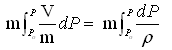                                       W₃ =                                   (4.3)

 

If the fluid is to flow from point B to point A at the standard state, then Eqn. (4.1) is the loss in potential energy, Eqn. (4.2) is the loss in kinetic energy, and Eqn. (4.3) is the loss in fluid-pressure energy (elastic energy).

 

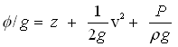
Fluid Potential (f) is the sum of W₁, W₂, and W₃ for unit mass of fluid (i.e., m = 1 in the above equations) as given below:

 

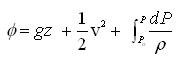                                         (4.4)

 

For incompressible fluid,  is constant. Thus, Eqn. (4.4) becomes

 

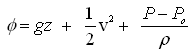                                    (4.5a)

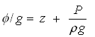
It is common in groundwater hydrology to set P_o equal to zero and work in gauge pressure (i.e., pressure above atmospheric).  That is, Eqn. (4.5a) can also be written as:

 

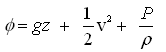                                          (4.5b)

 

The right hand terms of Eqns. (4.5a and 4.5b) indicate the total mechanical energy per unit mass of the fluid, i.e., fluid potential.

4.1.2 Relation between Fluid Potential and Hydraulic Head

After dividing Eqn. (4.5b) both sides by g (acceleration due to gravity), we have:

                                     (4.6)

 

Eqn. (4.6) indicates the total mechanical energy per unit weight of the fluid, which is known as hydraulic head (h). Hence, the right hand terms of Eqn. (4.6) can be replaced by h, and then Eqn. (4.6) reduces to:

 

                                                     (4.7)

 

That is, Fluid potential = Hydraulic Head × Acceleration due to gravity.

 

Note that Eqn. (4.6) expresses all the terms in units of energy per unit weight, which has the advantage of having all units in length dimensions.

 

For the flow through porous media, the flow velocity is very low, and hence the second term of Eqn. (4.6) is usually neglected. Then, Eqn. (4.6) can be written as follows:

 

                                                (4.8a)

 

Or,                                                            (4.8b)

 

Where, h = hydraulic head, z = elevation head, and h_p = pressure head.

 

Thus, hydraulic head (h) at any point in a porous medium is the sum of ‘elevation head’ and ‘pressure head’. Since pressure head is a function of space and time, and hence hydraulic head is also a function of space (x, y, z) and time (t). The ‘pressure head’ at a point in the saturated porous medium is measured by installing a tube or a small diameter pipe at that point. In the laboratory, the tube is called a ‘monometer’ and for the field, small diameter pipe is called a ‘piezometer'. The ‘elevation head’ is measured with respect to a datum (reference line), which is usually ‘mean sea level’ (MSL).

 

4.2 Darcy’s Law

Based on a laboratory experiment on a sand column, Henry Darcy in 1856 observed that the rate of flow (Q) through the sand column is directly proportional to the head loss over the column length (dh) and cross-sectional area (A), and is indirectly proportional to the column length (dl). That is,

 

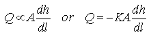                                 (4.9)

 

In Eqn. (4.9), the constant of proportionally (K) is known as the hydraulic conductivity of the porous medium. Sometimes K is also called saturated hydraulic conductivity of the porous medium because of the fact that the Darcy’s law is strictly valid for flow through a saturated porous medium. Negative sign in Eqn. (4.9) indicates that the flow occurs in the direction of decreasing head. The term   is the head loss per unit length of flow and is called hydraulic gradient (i). Equation (4.9) can also be written as follows:

 

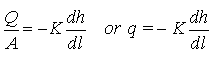                               (4.10)

Where, q is called Darcy velocity (Darcy flux) or specific discharge. Darcy velocity is a volume flux defined as the discharge per unit bulk area (including both pore space and solids) of a porous medium. Thus, Darcy velocity (q) is a macroscopic flux and in no case, it is equal to the displacement of fluid elements per unit time (usual meaning of velocity). Therefore, better terms like ‘Darcy flux’ or ‘specific discharge’ have been suggested by hydrogeologists and soil physicists instead of Darcy velocity.

 

Darcy’s law is widely used to quantity flow in aquifer systems. For example, if the Darcy flux in an aquifer is 0.1 m/day and the aquifer normal to the flow direction is 10 m thick and 1000 m wide, then the groundwater flow rate in the aquifer is: q×A = 0.1×10×1000 = 1000 m³/day. Groundwater discharge (flow rate) can also be calculated if the values of hydraulic conductivity (K), hydraulic gradient (i) and the area of an aquifer (A) are known.  

 

4.3 Validity of Darcy’s Law

The Darcy law is valid for the groundwater flow condition when head loss is directly proportional to the velocity of flow. Such a flow condition exists when the groundwater flow is laminar. That is, the Darcy law is valid for laminar flow only.

 

To check the validity of the Darcy law, a non-dimensional number called Reynolds Number is used. Reynolds Number (R_e) is given as:   

 

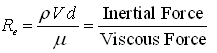                               (4.11)

 

Where, ρ = density of the fluid, V = flow velocity, d = characteristic length, and m = dynamic viscosity of the fluid.

 

For flow through porous media, V is usually taken as the Darcy velocity and d is better represented by d₁₀ (effective grain diameter/size of the porous media), though d is also taken as d₅₀ (mean or median grain diameter/size of the porous media) by some hydrogeologists.  

 

Experiments have shown that the Darcy’s law is strictly valid for R_e<1, but it doesn’t depart seriously up to R_e = 10 (Ahmed and Sunada, 1969). Hence, in practice, the Darcy’s law may be applied to flow conditions that exist when R_e≤10.  A range of values rather than a unique limit must be stated because as inertial forces in the tortuous paths of porous-media flow increase, turbulence occurs gradually (Todd, 1980). The irregular flow paths of eddies and swirls associated with the turbulence first occur in larger pores; with increasing velocity they spread to smaller pores. For the fully developed turbulence, the head loss (ΔH) varies approximately with the second power of the velocity (i.e., ΔH µV²) rather than linearly as in the case of laminar flow.

 

Fortunately, most natural groundwater flow occurs with R_e≤1, and hence the Darcy’s law is generally applicable. Deviations from the Darcy’s law can occur in some special situations where steep hydraulic gradients exist. For example, groundwater flow in the vicinity of pumping wells as well as turbulent flow in rocks having fractures, fissures and solution cavities/channels such as basalt and limestone that contain large underground openings.

 

Example Problem: A sand aquifer has an effective grain diameter of 0.2 mm. The density of groundwater is 1.003×10³ kg/m³ and its dynamic viscosity is 1.15×10^-3 N s/m² (kg/s m). If the rate of groundwater flow is 0.0016 m/s, check the validity of the Darcy’s law for this flow system.

 Solution: Reynolds number (R_e) is given as:

 

 

Here, r = 1.003×10³ kg/m³, v = 0.0016 m/s, d = 0.2 mm = 0.0002 m, and m = 1.15×10^-3 N s/m². Substituting these values in the above equation, we have

 

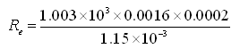
       =0.2791   , which is less than 1.

 

Therefore, Darcy’s law is valid for the given flow system.

 

4.4 Seepage Velocity

In reality, groundwater movement occurs through the conductive pores and cracks of the aquifer material only, and hence the actual velocity of groundwater is greater than the Darcy flux or specific discharge. The velocity of groundwater through the effective pores of a porous medium is called seepage velocity or groundwater velocity (sometimes also called “average linear velocity”), which is actual velocity of groundwater flow. Thus, actual groundwater discharge (Q) can be computed as follows:

 

                                         (4.12)

 

Where, n_e = effective porosity of the aquifer, V_s = seepage velocity or actual groundwater velocity, and the remaining symbols have the same meaning as defined earlier.

 

Equation (4.12) can also be written as:

 

                                             (4.13a)

 

Or,                                                                                            (4.13b)

 

Equation (4.13b) gives the relationship between the Darcy flux (specific discharge) and the seepage velocity. Obviously, the seepage velocity (actual groundwater velocity) can be computed by dividing the Darcy flux (q) with effective porosity (n_e).  For example, if the Darcy flux in an aquifer is 0.1 m/day and the effective porosity of the aquifer (n_e) is 12%, then the actual groundwater velocity will be: =. = 0.83 m/day, which is about eight times the Darcy velocity. Thus, the seepage velocity or actual groundwater velocity is always greater than the Darcy velocity.

 

4.5 Hydraulic Conductivity and Transmissivity

4.5.1 Hydraulic Conductivity

Hydraulic conductivity (K) of a saturated porous medium can be defined from Darcy’s law as:

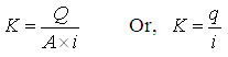                                    (4.14)

 

Where, K = hydraulic conductivity of the aquifer, Q = groundwater discharge (rate of groundwater flow), A = cross-sectional area of the aquifer, i = hydraulic gradient, and q = specific groundwater discharge or Darcy flux.

 

Thus, hydraulic conductivity (K) can be defined as ‘the groundwater discharge per unit cross-sectional area of the aquifer under a unit hydraulic gradient’. Alternatively, it can also be defined as ‘the specific groundwater discharge under a unit hydraulic gradient. K has the dimension of velocity (i.e., L/T).

 

The relationship between hydraulic conductivity (K) and intrinsic permeability (k) of a porous medium is given as follows (Todd, 1980):

 

                                               (4.15a)

 

Or,                                                                                             (4.15b)

 

Where, μ = dynamic viscosity of the groundwater,  ρ= density of the groundwater, g = acceleration due to gravity, and v = = kinematic viscosity of the groundwater.

 

It is clear from Eqn. (4.15a) that the hydraulic conductivity of a porous medium is dependent on the properties of both the porous medium and the fluid (liquid or gas) passing through it.  In groundwater hydrology, K is usually expressed in m/day which gives an easy understanding of groundwater flow because the movement of groundwater is normally slow.

 

4.5.2 Transmissivity

Transmissivity (T) of an aquifer system describes how transmissive an aquifer is in moving water through its pore spaces. It is defined as the product of hydraulic conductivity (K) and the saturated thickness (b) of the aquifer. That is,

 

                                                T = Kb                                                     (4.16)

 

Transmissivity of an aquifer system can also be defined from Darcy’s law as follows:

 

According to the Darcy’s law, we have:

 

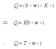
                                              (4.17)

 

Where, Q = groundwater flow rate (discharge), K = hydraulic conductivity of the aquifer, b = saturated thickness of the aquifer, w = width of the aquifer, i = hydraulic gradient, and T = transmissivity of the aquifer.

 

Thus, transmissivity can be defined as ‘the rate of groundwater flow through the entire saturated thickness of an aquifer of unit width under a unit hydraulic gradient’.

 

Note that the concept of transmissivity inherently assumes horizontal flow in aquifer systems. This concept can also be used for unconfined aquifers. In this case, b in Eqn. (4.16) is replaced with  (average saturated thickness of the unconfined aquifer) because of varying saturated thickness caused by the presence of free water surface (i.e., water table).

 

4.6 Leakage Factor

Leakage factor is a characteristic length of leaky aquifers. It is mathematically expressed as:

 

                                                                                        (4.18a)

 

Or,                                                                                         (4.18b)

 

Where, T = transmissivity of the aquifer, b’ = thickness of the leaky confining layer (aquitard), K’ = vertical hydraulic conductivity of the leaky confining layer (aquitard), and c= hydraulic resistance of the aquitard.

 

The leakage factor (B) has the dimension of length, i.e., [L]. Moreover, Leakance or Leakage Coefficient is defined as . The numerical values of leakance are usually given as a measure of leakage rates (i.e., ability of the aquitard to transmit vertical flow through it). Leakance has the dimension of time inverse (e.g., day^-1).

 

References

Ahmed, N. and Sunada, D.K. (1969). Nonlinear flow in porous media. Journal of Hydraulics Division, ASCE, 95(HY6): 1847-1857.

Todd, D.K. (1980). Groundwater Hydrology. John Wiley & Sons, New York.

Suggested Readings

Todd, D.K. (1980). Groundwater Hydrology. John Wiley & Sons, New York.

Fetter, C.W. (2000). Applied Hydrogeology. 4th Edition. Prentice Hall, NJ.

Sarma, P.B.S. (2009). Groundwater Development and Management. Allied Publishers Pvt. Ltd., New Delhi.