Irrigation Engineering 4(3+1)

LESSON 5 Methods of Water Measurements in Open Channels

Water may be measured in two condition viz. (i) at rest and (ii) in motion. At rest means volume of water is measured and different units used for volume measurement are litre, cubic metre, hectare-centimetre, hectare-metre etc.Water is measured in motion means rate of flow is measured and different units used for this are litre per second, cubic metre per second, etc.

1. Litre: The volume equal to one cubic decimetre or 1/1000 cubic metre.
2. Cubic metre: A volume equal to that of a cube 1 metre long, 1 metre wide and 1 metre deep.
3. Hectare – centimetre: A volume necessary to cover an area of 1 hectare (10,000 sq.m) up to a depth of 1 centimetre (1 hectare – centimetre = 100 cu. m = 100,000 litres)
4. Hectare –metre: A volume necessary to cover 1 hectare (10,000 sq.m) up to a depth of 1 metre (1 hectare –meter = 10,000 cu. m = 10 M litres)
5. Litre per second: A continuous flow amounting to 1 litre passing through a point each second.
6. Cubic metre per second: A flow of water equivalent to a stream 1 metre wide and 1 metre deep, flowing at a velocity of 1 metre per second.

 

5.1.1 Methods of Water Measurements

There are several methods used for the measurements of irrigation water on the farm. They can be grouped into four categories as,

1. Volumetric or volume methods of water measurement
2. Area – Velocity Method
3. Measuring Structures (Orifices, Weirs and Flumes)
4. Tracer methods.

 

5.2 Volume Methods of Water Measurement

This method is suitable for measuring small irrigation stream. In this case, water is collected in a container of known volume and the time taken to fill the container is recorded. The rate of flow is measured by the formula

 

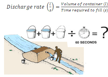
 5.1.Volume Method.(Source:ftp://ftp.fao.org/fi/CDrom/FAO_Training/FAO_Training/General/x6705e/x6705e03.htm)

 

5.2.1 Area-velocity Method

The rate of flow of water passing a point in open channel is determined by multiplying the cross sectional area of the flow section at right angles to the direction of flow by the average velocity of water. The cross sectional area is determined by measuring the depths at various locations. The depth can be measured by different methods like sounding rods or sounding weights or echo-depth sounder for accurate measurement.

For discharge calculation the entire cross section is divided into several subsections and the average velocity at each of these sub-sections is determined by current meters or floats. The accuracy of discharge measurement increases with the increase in the number of segments. Some guidelines for choosing the number of sections are:

a) The discharge in the segment should not be more than 10% of total discharge.

b) The difference in velocities between two adjacent sections should not be more than 20%.

c) The segment width should not 1/15^th to 1/20^th of total width.

 

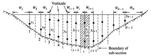
Fig.5.2.Stream section for area velocity method.

(Source: Subramanya, 1994)

Calculation of Discharge

The total discharge is calculated using the method of mid sections. It has been considered that the section is divided into N-1 sections.

                                                                                                 .......(5.2)

Where,

ΔQ_i= discharge in i^th section.

= (depth at i^th section) x (½ width to the left + ½ width to the right) X  (average velocity in the i^th section)

                                                                                                     ..............(5.3)

 For the fist and last sections, the area is calculated as:

                                                                                                        .........(5.4) 

where,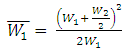        

                                                                                                                                          ........(5.5)                                 

and        

                                                                                                                                          .......(5.6)                            

Similarly   

                                                                                                                                          ...........(5.7)                          

 

Fig.5.3. Discharge measurement at a section.

(Source:http://serc.carleton.edu/microbelife/research_methods/environ_sampling/streamgage.html accessed on 05/0602012)

 

The cross sectional area is determined as discussed above and velocity is generally measured with a current metre. Approximate values of velocity may also be obtained by the float method. The detailed description of current meter method is given in section 5.2.2.

 5.2.1.1 Float Method

It is inexpensive and simple. This method measures surface velocity. Mean velocity is obtained using a correction factor. The basic idea is to measure the time that it takes for the object to float a specified distance downstream.

 

V_surface= travel distance/ travel time = L/t                                                 .........(5.8)

             Because surface velocities are typically higher than mean or average velocitie

V _mean = k .V_surface        

                                                                                                                                                                                     _{..................(5.9)}                                  

Where,

k is a coefficient that generally ranges from 0.8 for rough beds to 0.9 for smooth beds (0.85 is a commonly used value).

Step 1- Choose a suitable straight reach with minimum turbulence (ideally at least 3 channel widths long).

Step 2 - Mark the start and end point of your reach.

Step 3 - If possible, travel time should exceed 20 seconds.

Step 4 - Drop your object into the stream upstream of your upstream marker.

Step 5 - Start the watch when the object crosses the upstream marker and stop the watch when it crosses the downstream marker.

Step 6 -You should repeat the measurement at least 3 times and use the average velocity in further calculations.

 

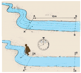
Fig.5.4. Float Method

(Source:ftp://ftp.fao.org/fi/CDrom/FAO_Training/FAO_Training/General/x6705e/x6705e03.htm)

 

 

5.2.2 Current Meters

In the area velocity method current meters are generally used to measure the velocity of flow at the different sections. The current meter consists of a small revolving wheel or vane that is turned by the movement of water. It may be suspended by a cable for measurements in deep streams or attached to a rod in shallow streams. The propeller is rotated by the flowing water and speed of propeller is proportional to the average velocity of flow. Corresponding to the number of revolutions, the velocity can obtained from calibration graphs or tables.

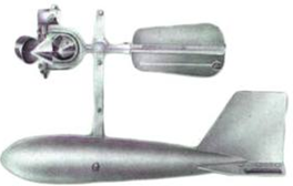
Fig. 5.5.Current meter.

(Source:http://www.weatherstation.co.in/full-images/730336.jpg: accessed on June 18, 2013)

 

Procedure for velocity measurement using the current meter:Stretch a tape across the channel cross-section. Divide the distance across the channel to at least 25 divisions. Use closer intervals for the deeper parts of the channel.

1. Stretch a tape across the channel cross-section. Divide the distance across the channel to at least 25 divisions. Use closer intervals for the deeper parts of the channel.
2. Start at the water’s edge and call out the distance first, then the depth and then the velocity. Stand downstream from the current meter in a position such that the velocity is least affected by the meter. Hold the rod in a vertical position with the meter directly into the water.
3. To take a reading, the meter must be completely under water, facing the current, and free of interference. The meter may be adjusted slightly up or downstream to avoid boulders, snags and other obstructions. The note taker will call out the calculated interval, which the meter operator may decide to change (e.g., taking readings at closer intervals in deep, high-velocity parts of the channel). Record the actual distance called out by the meter operator as the center line for the subsection.
   
   • Take one or two velocity measurements at each subsection.
   • If depth (d) is less than 60 cm, measure velocity once for each subsection at 0.6 times the total depth (d) measured from the water surface.
   • If depth (d) is greater than 60 cm, measure velocity twice, at 0.2 and 0.8 times the total depth. The average of these two readings is the velocity for the subsection.
4. Allow a minimum of 40 seconds for each reading. The operator calls out the distance, then the depth, and then the velocity. The note taker repeats it back as it is recorded, as a check.
5. Calculate discharge in the field. If any section has more than 5% of the total flow, subdivide that section and make more measurements.
   

 

Current meters are designed in a manner such that the rotation speed of the blades varies linearly with the stream velocity. This can be expressed by the following equation:

                                  v = a N _s + b                             ................(5.10)

 

Where,

v = stream velocity at measuring site in m/s

N_s = revolutions per second of the meter

a, b = constants of the meter.

To determine the constants, which are different for each instrument, the current meter has to becalibrated before use. This is done by towing the instrument in a tank at a known velocity and recording the number of revolutions N_s. This procedure is repeated for a range of velocities.

It has to be kept in mind that for shallow streams the measurement can be taken at a depth= 0.6 of the total depth, whereas for deeper streams two measurements are needed at 0.2 and 0.8 of total depth and then averaged to get the actual velocity.

 

Example 5.1:

Data pertaining to a stream-gauging operation at a gauging site are given below. The rating equation of the current meter is v = 0.63N_s + 0.08m/s. where N_s = revolutions per second. Calculate the discharge in the stream.

 

Distance from the left water edge (m)	0	5.0	8.0	11.0	14.0	17.0	20.0	24.0
Depth (m)	0	1.8	3.4	4.6	3.7	2.6	1.5	0
Revolutions of a current meter kept at 0.6 depth	0	42	55	93	87	48	28	0
Duration of observation (s)	0	120	120	125	135	110	100	0

 

Solution:

For the last and first section using equation

Average width,

 

For the rest of the segments, 

 

Since the velocity is measured at 0.6 depth the measured velocity is the average velocity at that vertical

The calculation of discharge is shown below:

Distance from the left water edge (m)	Average width  (m)	Depth y (m)	Ns = rev. /sec	Velocity  (m/s)	Segmental discharge  (m3/s)
0	0	0			0.0000
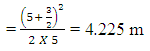
5	4.225	1.8	0.350	0.3005	2.2853
8	3	3.4	0.458	0.3688	3.7613
11	3	4.6	0.744	0.5487	7.5723
14	3	3.7	0.644	0.4860	5.3946
17	3	2.6	0.436	0.3549	2.7683
20	4.225	1.5	0.280	0.2564	1.6249
24	0	0			0.0000
Sum         = 23.4067

∴ Discharge in the stream = 23.40 m³/s Ans.

 

5.2.3 Other Method

5.2.3.1Tracer Method

In the tracer-dilution methods, a tracer solution is injected into the stream at one point and the tracer is measured at a point downstream to the first point. Knowing the rate and concentration of tracer in the injected solution and the concentration in the downstream section, the stream discharge can be computed.Either constant rate injection method or sudden injection method may be used for determining the discharge of a stream by tracer dilution.

Constant rate injection method: In this method the tracer solution is injected at a constant rate into the stream till a constant concentration of the tracer in the stream flow at the downstream sampling cross section is achieved. Fig. 5.6 shows constant rate injection system.

 

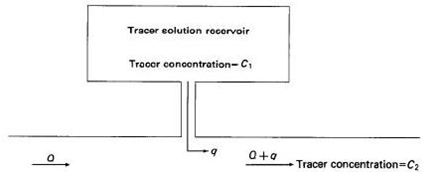
Fig.5.6.Constant rate injection system.

(Source: Measurement and Computation of Stream flow:  Volume 1. Measurement of Stage and Discharge - USGS)

If the tracer is injected for a sufficiently long period, sampling of the stream at the downstream sampling cross section will produce a concentration-time curve similar to that shown in Fig. 5.7.

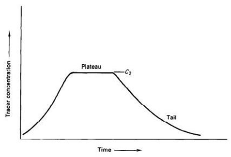
Fig. 5.7.Concentration-time curve at downstream sampling site for constant-rate injection.

(Source: Measurement and Computationof Stream flow:  Volume 1. Measurement of Stage and Discharge - USGS)

 

The stream discharge is computed from the equation for the conservation of mass, which follows:

      

                                                                                                                                                                                              ...........(5.11)

 

                                                                                                                                                                                                    .........(5.12)

 

Where,

q is the rate of flow of the injected tracer solution,

Q is the discharge of the stream,

C_b is the background concentration of the stream,

C₁ is the concentration of the tracer solution injected into the stream, an 

C₂ is the measured concentration of the plateau of the concentration-time curve (Fig. 5.7).

 

Example 5.2:

A 12g/L solution of a tracer was discharged into a stream at a constant rate of 15 cm³ s^-1. The background concentration of the dye in the stream water was found to be 2 parts per billion. At a downstream location sufficiently far away, the dye was found to reach an equilibrium concentration 7 parts per billion. Estimate the stream discharge.

 

Solution:

From equation 5.12 we know the stream discharge, 

 

 

 Given: q = 15 cm³ /s = 15 x 10^-6 m³ s-¹

 C₁ = 0.012, C₂ = 7 x 10^-9, C_b = 2 x 10^-9

 Putting the above values in the equation,

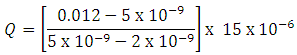
= 60 m³ /s

∴ Discharge through the stream = 60 m³ /sAns.

 

References

Bruckner, Z. M., Stream Gaging Using the Velocity-Area Method, Montana State University,Bozeman.

Measurement and Computation of Stream flow:  Volume 1. Measurement of Stage and Discharge – USGS

Rantz, S. E. (1982). Measurement of Streamflow: Measurement and Discharge and Computation Volume of Stage, Geological Survey Water-supply Paper 2175, USGS

Subramanya, K. (1994). Engineering Hydrology, Tata McGraw-Hill Education, New Delhi.

 

Internet References

http://serc.carleton.edu/microbelife/research_methods/environ_sampling/streamgage.html

http://ga.water.usgs.gov/edu/streamflow2.html

http://ga.water.usgs.gov/edu/

 

Suggested Readings:

Measurement and Computation of Stream flow:  Volume 1. Measurement of Stage and Discharge – USGS

Rantz, S. E. (1982). Measurement of Streamflow: Measurement and Discharge and Computation Volume of Stage, Geological Survey Water-supply Paper 2175, USGS.

Subramanya, K.(1994). Engineering Hydrology, Tata McGraw-Hill Education.