Soil & Water Conservation Engg. 3(2+1)

Lesson 18 Estimation of USLE Parameters

18.1 USLE Parameters

However, USLE predicts only the amount of soil loss that results from sheet or rill erosion on a single slope and does not account for additional soil losses that might occur from gully, wind or tillage erosion.

Five major factors are used to calculate the soil loss for a given site. Each factor is the numerical estimate of a specific condition that affects the severity of soil erosion at a particular location. The erosion values reflected by these factors can vary considerably due to varying weather conditions. Therefore, the values obtained from the USLE more accurately represent long-term averages.

USLE has been found to produce realistic estimates of surface erosion over areas of small sizes (Wischmeier & Smith, 1978). Therefore, soil erosion within a grid cell was estimated using the USLE. The USLE is expressed as:

A = gross amount of soil erosion (t ha^-1 yr^-1); it represents the potential long term average annual soil loss in tons per hectare per year. This is the amount, which is compared to the "tolerable soil loss" limits, R = rainfall factor related to rainfall-runoff erosion given in MJ.mm.ha^-1h^-1, K = soil erodibility factor related to soil erosion (t.ha.h.MJ^-1 mm^-1), L = slope length factor (dimensionless), S = slope steepness factor (dimensionless), C = factor related to cover management (dimensionless); and P = conservation practice factor (dimensionless).

18.1.1 Description of Different Parameters of USLE

Rainfall Factor (R)

The erosivity factor to account for the erosive power of rainfall is related to the amount and intensity of rainfall over the year (erosivity index unit). Rainfall erosivity is a term used to describe the potential for soil to be washed off from disturbed, devegetated areas into surface waters during storms. The potential for erosion is based on many factors which include soil type, slope, and the energy or force of precipitation expected during the period of surface disturbance.

Soil Erodibility Factor (K)

The soil erodibility factor to account for the soil loss rate is an erosion index unit which is defined as the soil loss from a plot 22.1 m long on a 9% slope under a continuous bare cultivated fallow. It ranges from less than 0.1 for the least erodible soils to close to 1.0 in the worst possible case.

Topographic Factor (LS)

LS is the slope length-gradient factor. The topographic factor is used to account for the length and steepness of the slope. The longer the slope, the greater is the volume of surface runoff and the steeper the slope, the greater is its velocity. LS is 1.0 on a 9% slope and for a 22.1 meter long plot.

Crop Management Factor (C)

C is the crop/vegetation and management factor. It is used to determine the relative effectiveness of soil and crop management systems in terms of preventing soil loss. The C factor is a ratio of the soil loss from a land under a specific crop and management system to the corresponding loss from a continuously fallow and tilled land. The C Factor can be determined by selecting the crop type and tillage method.

The cover and management factor to account for the effects of vegetative cover and management techniques for reduction of the soil loss would be equal to 1.0 in the worst case. In an ideal case when there is no sediment loss, C would be zero.

Support Practice Factor (P)

P is the support practice factor. It reflects the effects of practices that will reduce the amount and rate of the runoff and thus reduce the amount of erosion. The P factor represents the ratio of soil loss by a support practice to that of straight-row farming up and down the slope. The most commonly used supporting cropland practices are cross slope cultivation, contour farming and strip-cropping. Ideally in an area with full support practice condition, P would be zero meaning there is no sediment loss; whereas in an area without any support practice P = 1.0 indicating maximum possible sediment loss in absence of any soil conservation practice.                                                                              

18.2 Assumptions and Estimation of USLE Parameters

Wischmeier (1976) reported that the USLE may be used to predict the average-annual soil loss from a field-sized plot with specified land use conditions (Mitchell and Bubenzer 1980). The assumptions associated with the USLE are as follows (Goldman et. al. 1986; Novotny and Chesters 1981; Foster 1976; Onstad and Foster 1975):

• The USLE is an empirically derived algorithm and does not mathematically represent the actual erosion process.

• The USLE was developed to estimate long-term, average-annual, or seasonal soil loss. Unusual rainfall seasons, especially higher than normal rainfall and typically heavy storms may produce more sediment than estimated.

• The USLE estimates soil loss on upland areas only; it does not estimate sediment deposition. Sediment deposition generally occurs at the bottom of a slope (i.e., change in grade) where the slope becomes milder.

• The USLE estimates sheet, rill, and inter-rill erosion and does not estimate channel or gully erosion.  Gully erosion, caused by concentrated flows of water, is not accounted for by the equation and yet can produce large volumes of eroded soil.

• The USLE was developed originally to address soil loss from field-sized plots, although with proper care, watersheds can be addressed.

• Because the USLE only estimates the volume of sediment loss (i.e., the volume of soil detached and transported some distance), it can be used to estimate sediment transport capacity at a site.

• Because the USLE represents an empirically derived expression, consistently accurate estimates of soil loss are fortuitous at best.

• The USLE does not estimate soil loss from single storm events unless a modified form of the original equation is used.

18.2.1 Estimation of USLE Parameters

1. Rainfall Erosivity (R)

The following two methods are widely used for computing the erosivity of rainfall.

a) EI₃₀ index method.

b) KE > 25 index method.

a) EI₃₀ Index Method

This method was introduced by Wischmeier (1965). It is based on the fact that the product of kinetic energy of the storm and the 30-minute maximum rainfall intensity gives the best estimation of soil loss. The greatest average intensity experienced in any 30 minute period during the storm is computed from recording raingauge charts by locating the maximum amount of rain which falls in 30 minute period and later converting the same to intensity in mm/hour. This measure of erosivity is referred to as the EI₃₀ index and can be computed for individual storms, and the storm values can be added over periods of time to give weekly, monthly or yearly values of erosivity.

The rainfall erosivity factor EI₃₀ which gives R value is computed as follows:

where KE is the rainfall kinetic energy and I₃₀ is the rainfall intensity for a 30-minute period. Kinetic energy for the storm is computed using Eqn.17.1.

Limitation

The EI₃₀ index method was developed under American conditions and is not found suitable for tropical and subtropical zones for estimating the erosivity.

b) KE > 25 Index Method

This is an alternate method introduced by Hudson for computing the rainfall erosivity of tropical storms. This method is based on the concept that, erosion takes place only at threshold value of rainfall intensity. From experiment, it was obtained that rainfall intensity less than 25 mm/h are not able to cause soil erosion in significant amount. Thus, this method takes care of only those rainfall intensities, which are greater than 25 mm/h. Due to this reason, it is named as K.E.> 25 index method.

Calculation Procedure

The estimation procedure is same for both the methods. However, K.E.> 25 method is more advantageous, because it sorts out all the data with rainfall intensity of less than 25 mm/h and therefore, requires less rainfall data. For application of both the methods it is essential to have data on rainfall amount and intensity.

The procedure involves multiplication of rainfall amounts in each class of intensity to the computed kinetic energy values and then all these values are added together to get the total kinetic energy of storm. The K.E. so obtained is again multiplied by the maximum 30-minute rainfall intensity, to determine the rainfall erosivity value.

2. Soil Erodibility (K)

Erodibility of a soil is designated by the soil erodibility factor K. The formula used for estimating K is as follows:

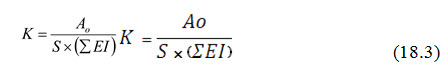
where,  K = soil erodibility factor, A_o = observed soil loss, S = slope factor and  ∑EI = total rainfall erosivity index.

Although several techniques are available to determine the value of K, three important approaches are discussed below.

1. Use of In Situ Erosion Plots

2. Measuring K under a Simulated Rainstorm

3. Predicting K using Regression Equations Describing the Relationship between K and Soil Physical and Chemical Properties.

1. In Situ Erosion Plots

Erosion plots enable measurement of K under field conditions. They make use of a standard condition of bare soil, no conservation practice and 7° slope of 22m with 22 m length of plot. This approach is costly and time consuming.

2. Measuring K under a Simulated Rainstorm

This approach is less time consuming but relatively costly. The main drawback is that none of the rainfall simulators built to date can recreate all the properties of natural rain. Nevertheless this method is being used more extensively in erosion studies.

The rainfall simulator used in this study is made of Duction bars and measures 1.80 m by 1.80 m and 3.80 m high. Several kinds of nozzles are tested and the one that produces water droplets close to natural rain is chosen. Water is released at a low pressure. A wooden tray of dimension 1 m by 2 m and 15 cm deep is placed under the simulator with the slope adjusted to 7°. The tray is properly packed with the test soil. A collecting structure is placed at the down slope end to gather runoff and sediment. Soil samples are collected from different erosion-sensitive regions placed in the wooden tray.

The soil is then subjected to simulated rainstorm of different intensities. Since, it is difficult to set a predetermined rainfall intensity, the nozzle is adjusted to low and high levels and the depth of water reaching the wooden tray is measured throughout the experiment using a beaker. For all the experiments, runoff and sediments are collected and measured.

3. Predicting K using Regression Equations

K may be predicted using regression equations describing the relationships between K and soil chemical and physical properties. The nomograph developed by Wischmeier et al. (1971) expressing the relationship between K and soil properties is based on the following equation:

where OM = organic matter content (%), m = silt plus fine sand content (%), St = soil structure code (very fine granular = 1, fine granular = 2, coarse granular = 3, blocky, platy or massive = 4), Pt  = permeability class (rapid = 1, moderate to rapid = 2, moderate = 3, slow to moderate = 4, slow = 5, very slow = 6 ). Based on the above equation, Wischmeier et al. (1971) developed a nomograph which is used to predict K. 

3. Topographic Factor (LS)

Slope length factor (L) is the ratio of soil loss from a 22.13 m length plot under identical conditions. The soil loss has a direct relationship with the slope length i.e., it is approximately proportional to the square root of the slope length (L^0.5).

Steepness of land slope factor (S) is the ratio of soil loss from the existing field slope gradient to that from the 9% slope under otherwise identical conditions. The increase in steepness of slope results in the increase in soil erosion as because the velocity of runoff increases with the increase in field slope allowing more soil to be detached and transported along with surface flow.

The two factors L and S are usually combined into one factor LS called topographic factor. This factor is defined as the ratio of soil loss from a field having specific steepness and length of slope (i.e., 9% slope and length 22 m) to the soil loss from a continuous fallow land. The value of LS can be calculated by using the formula given by Wischmeier and Smith (1962):

where, L = Field slope length in feet and S = percent land slope.

Wischmeier and Smith (1978) based on the observations from crop land on slopes ranging from 3 to 18% and length from 10 to 100 m, derived the following equation for LS factor in M.K.S. system .

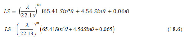
where, λ = field slope length in meters, m = exponent factor varying from 0.2 to 0.5 and θ = angle of slope.

Mc Cool et al. (1987) further modified the slope steepness factor for use in USLE, described as under.

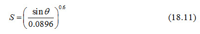
• For Shorter Slopes not greater than 4 m

For this specific condition, the S can be predicted by the following equation:

where, θ = the angle of slope and  S = percent land slope.

• For Longer Slopes

From an analysis, two relationships were derived. One is applicable to slopes less than 9% and the other one for slopes equal to or greater than 9%. The revised equations are as follows:

•  Slope less than 9%

      S = 10.8 Sin θ + 0.03                                     (18.8)

•  Slope equal to or greater than 9%

     S = 16.8 Sin θ - 0.50                                       (18.9)

These equations apply best to relatively smooth surfaces, where tillage is up and down the hill and runoff does not vary with the slope for steepness above 8%.

• For the condition, where erosion is mainly caused by surface flow overthrowing the soil, the following equations for S have also been developed.

(a)   Slope less than 9%

     S = 10.8 Sin θ + 0.03                                     (18.10)

(b)  Slope equal to greater than 9%

4. Crop Management Factor, C

This is an important factor of USLE, because it accounts for the condition that can be easily managed on soil to reduce the erosion. The value of C is determined as a weighted average of soil loss ratios (SLRs), defined as the ratio of soil loss for a given condition of vegetative cover at a specific time to that of the unit plot soil loss. As per this the definition, the SLRs vary within a year duration, as the soil cover conditions are likely to change appreciably during a year. To obtain the C value, the SLRs are weighted according to the erosivity distribution during the entire year.

To compute SLRs, a sub- factor method is introduced, which is a function of four sub-factors as given below:

1. Prior land use sub-factor (PLU)

2. Crop canopy sub-factor (CC)

3. Surface cover sub-factor (SC)

4. Surface roughness sub- factor (SR)

The sub-factor relationship is given as under:

The values of sub-factors PLU and SR for soil effect, are determined with the help of existing bio-mass amount in the soil that is accumulated from the crop’s root and incorporation of crop residues. For computation of sub-factor value for SLRs, the characteristics of tillage operation play an important role.

The surface roughness factor SC is determined based on the effect of surface ground cover on erosion as given by equation (18.13).

where, b = coefficient, assigned as 0.035. Its value increases as the tendency   of rill erosion to dominate inter rill erosion increases and M = percentage of ground cover.

5. Conservation Practices Factor, P

To determine the conservation practice factor, entire area can be divided into three categories,

1. Straight rows

2. Straight rows with grassed waterways

3. Terraces

Then the following equation is used to estimate P:

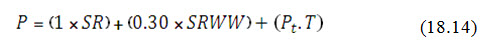
Where, SR is the portion of area under straight rows. SRWW is the portion of area under straight rows and grassed waterways; P_t is the erosion control practice for terracing and T is referred as the terraced area.

Keywords: USLE, Erodibility, Erosivity, Soil Loss.

References

Murty, V.V.N. (1985). Land and Water Management Engineering, Kalyani publishers, pp. 432-447.

Suresh, R. (2007). Soil and water conservation engineering, Second Edition, Standard Publishers Distributors, New Delhi, pp. 641-674.

Wischmeier, W.H., Johnson, C.B. and Crors, B.V. (1971). A soil erodibility nomograph for farmland and construction sites, Journal of soil and water conservation 26: pp.189-193.

Suggested Readings

Wischmeier, W.H., and Smith, D.D., 1978, Predicting Rainfall Erosion Losses - A Guide to Conservation Planning, U.S. Department of Agriculture, Agriculture Handbook No. 537.

Arnoldus, H.M.J., 1980, An approximation of the rainfall factor in the universal soil loss equation, In: De Boodt, M. and Gabriels, D. (Eds) Assessment of Erosion. John Wiley and Sons, Chichester, pp. 127-132.

Moore I, Burch G. 1986a, Physical basis of the length-slope factor in the Universal Soil Loss Equation, Soil Science Society of America Journal 50: pp. 1294–1298.

www.docstoc.com/docs/7676136/Introduction-General-Assumptions

www.omafra.gov.on.ca/english/engineer/facts/00-001.htm.