Watershed Hydrology 3(2+1)

Lesson 23 Base Flow Separation

There are three methods of base-flow separation that are in common use.

23.1.1. Method 1

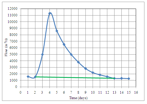
In this method the separation of the base flow is achieved by joining with a straight line the beginning of the surface runoff to a point on the recession limb representing the end of the direct runoff.

 

In Fig. 23.1, pointA represents the beginning ofthe direct runoff off and it is usually easy to identify in view of the sharp change in the runoff rate at that point. Point B, marking the end of the direct runoff is rather difficult to locate exactly.

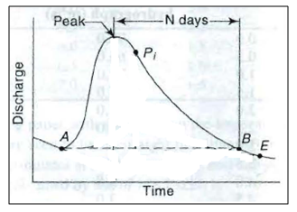
Fig. 23.1. Method 1 for base flow separation.(Source:Subramanya, 2008)

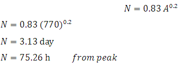
An empirical equation for the time interval N (days) from the peak to the point B is

 (23.1)

WhereA is drainage area in km²and N is in days. Points A and B are joined by a straight line to demarcate to the base flow and surface runoff. This method of base-flow separation is the simplest of all the three methods.

 

23.1.2 Method 2

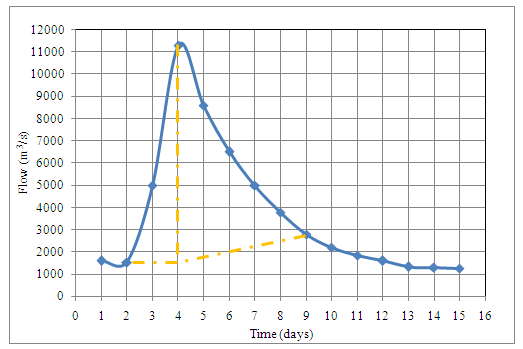
In this method the base flow curve existing prior to the commencement of the surface runoff is extended till it intersects the ordinate drawn at the peak (point C in Fig. 23.2). This point is joined to point B by a straight line. Segment AC and CB demarcate the base flow and surface runoff. This is probably the most widely used base-flow separation procedure.

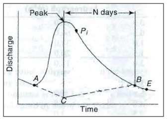
Fig. 23.2. Method 2 for base flow separation. (Source:Subramanya, 2008)

 

23.1.3 Method 3

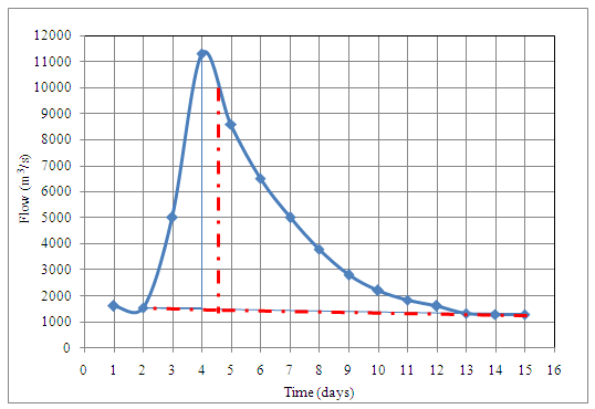
In this method the base flow recession curve after the depletion of the flood water is extended backwards till it intersects the ordinate at the point of inflection (line EF in Fig. 23.3). Points A and F are joined by an arbitrary smooth curve. This method of base-flow separation is realistic in situations where the groundwater contributions are significant and reach the stream quickly.

Fig. 23.3. Method 3 for base flow separation. (Source:Subramanya, 2008)

The surface runoff hydrograph obtained after the base-flow separation is also known as direct runoff hydrograph (DRH).

 

Example 1

The following are the ordinates of the hydrograph of flow from a catchment area of 770 km² due to a 6-h rainfall. Derive the ordinates of DRH. Make suitable assumptions regarding the base flow.

Time from beginning of storm	(h)	0	6	12	18	24	30	36
Discharge	(m3/s)	42	65	215	360	400	350	270
Time from beginning of storm	(h)	42	48	54	60	66	72
Discharge	(m3/s)	205	145	100	70	50	42

 

Answer:

Given: catchment area (A) = 770 km²

Using equation 23.1,

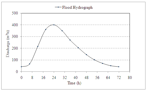
From given data, with our convenience, base flow = 42 m³/s at 72 h

Therefore, DRH = Flood Hydrograph – Base flow

 

Time from beginning of storm	Discharge	Base flow	DRH
h	m3/s	m3/s	m3/s
0	40	42	-2
6	65	42	23
12	215	42	173
18	360	42	318
24	400	42	358
30	350	42	308
36	270	42	228
42	205	42	163
48	145	42	103
54	100	42	58
60	70	42	28
66	50	42	8
72	42	42	0

Example 2

The daily stream flow data at a site having a drainage area of 6500 km² are given in the following table. Separate the base flow using the above three methods.

Time (days)	Discharge (m3/s)
1	1600
2	1550
3	5000
4	11300
5	8600
6	6500
7	5000
8	3800
9	2800
10	2200
11	1850
12	1600
13	1330
14	1300
15	1280

 

Answer

1. Plot the total runoff hydrographMethod 1: join point A, the beginning of direct runoff, to point B, the end of direct runoff. Both points are selected by judgment.

 2. Method 2: Extend the recession curve before the storm up to point C below the peak. Join point C to D, computed using equation

 3. Method 3: Extend the recession curve backward to point E. Join point E to A

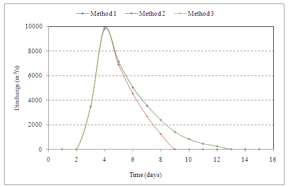
 4. The ordinates DRH by three methods are given in Table

Table Ordinates of DRH by different methods

Time	Total runoff	Base flow			Direct runoff
		Method 1	Method 2	Method 3	Method 1	Method 2	Method 3
(days)	(m3/s)	(m3/s)	(m3/s)	(m3/s)	(m3/s)	(m3/s)	(m3/s)
1	1600	1600	1600	1600	0	0	0
2	1550	1550	1550	1550	0	0	0
3	5000	1520	1480	1500	3480	3520	3500
4	11300	1500	1400	1450	9800	9900	9850
5	8600	1450	1700	1400	7150	6900	7200
6	6500	1450	1950	1400	5050	4550	5100
7	5000	1450	2300	1400	3550	2700	3600
8	3800	1400	2550	1400	2400	1250	2400
9	2800	1380	2800	1380	1420	0	1420
10	2200	1380	2200	1380	820	0	820
11	1850	1380	1850	1380	470	0	470
12	1600	1350	1600	1350	250	0	250
13	1330	1330	1330	1330	0	0	0
14	1300	1300	1300	1300	0	0	0
15	1280	1280	1280	1280	0	0	0

 

23.2 Effective Rainfall Hyetograph

Effective rainfall (also known as Excess rainfall) (ER) is that part of the rainfall that becomes direct runoff at the outlet of the watershed. It is thus the total rainfall in a given duration from which abstractions such as infiltration and initial losses are subtracted.

 

For purposes of correlating DRH with the rainfall which produced the flow, the hyetograph of the rainfall is also pruned by deducting the losses. Figure 23.4 shows the hyetograph of a storm. The initial loss and infiltration losses are subtracted from it. The resulting hyetograph is known as effective rainfall hyetograph (ERH). It is also known as excess rainfall hyetograph.

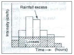
Fig. 23.4.Effective rainfall hyetograph. (Source:Subramanya, 2008)

Both DRH and ERH represent the same total quantity but in different units. Since ERH is usually in cm/h plotted agains1 time, the area of ERH multiplied by the catchment area gives the total volume of direct runoff which is the same as the area of DRH. Theinitial loss and infiltration losses are estimated based on the available data of the catchment.

 

Example 3

A 4-hour storm occurs over an 80 km² watershed. The details of the catchment are as follows:

Sub Area	Φ index	Hourly rain (mm)
km2	mm/h	1st hour	2nd hour	3rd hour	4th hour
15	10	16	48	22	10
25	15	16	42	20	8
35	21	12	40	18	6
5	16	15	42	18	8

 

Calculate the runoff from catchment and the hourly distribution of the effective rainfall whole catchment.

Answer:

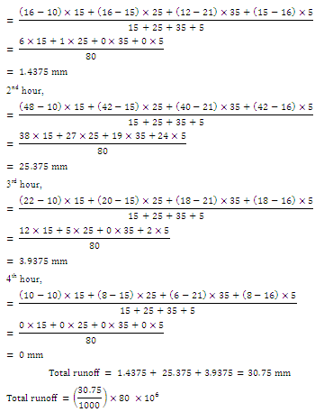
Totalrunoff = 2.46Mm³

Hourly distribution of the effective rainfall for the whole catchment:

	Effective rainfall (mm)
1st hour	1.4375
2nd hour	25.375
3rd hour	0
4th hour	3.9375

 

Example 4

A storm in a certain catchment had three successive 6-h intervals of rainfall magnitude of 3.0 cm, 5.0 cm and 4.0 cm, respectively. The flood hydrograph at the outlet of the catchment resulting from this storm is as follows:

Time	(h)	0	6	12	18	24	30	36	42
Flood hydrograph ordinates	(m3/s)	30	480	2060	4450	6010	6010	5080	3996
Time	(h)	48	54	60	66	72	78
Flood hydrograph ordinates	(m3/s)	2866	1866	1060	500	170	30

 

If the area of the catchment is 8791.2 km², estimate the index of the storm. Assume the base flow as 30 m³/s.

 

Answer

Flood hydrograph ordinates = DRH ordinates +Base flow ordinates

Direct runoff(cm) =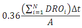 

Where

is direct runoff ordinates (m³/s),  is time interval between successive ordinates (h), A is catchment area (km²)

Time	Flood hydrograph Ordinates	Base flow	DRO
h	m3/s	m3/s	m3/s
0	30	30	0
6	480	30	450
12	2060	30	2030
18	4450	30	4420
24	6010	30	5980
30	6010	30	5980
36	5080	30	5050
42	3996	30	3966
48	2866	30	2836
54	1866	30	1836
60	1060	30	1030
66	500	30	470
72	170	30	140
78	30	30	0
		= 34188

 

Therefore,

Direct runoff (cm) = 

Directrunoff (cm)  = 8.4

Therefore

φ = 0.2cm/h 

 

 

Rainfall (cm)	3	5	4
Time interval (h)	6	6	6
Rainfall intensity (cm/h)	0.5	0.833	0.667
index (cm/h)	0.2	0.2	0.2
Excess rainfall intensity	0.3	0.633	0.467

 

23.3 Elemental Hydrograph

If a small, impervious area is subjected to a constant rate rainfall, the resulting runoff hydrograph will appear much as above, and is known as elemental hydrograph (Fig. 23.5). In the beginning, there will be surface detention (rainfall-runoff) so as to start the sheet flow over the surface. At point B, known as point of equilibrium, outflow rate equals inflow rate. When rainfall ends (at C), recession starts, i.e., outflow rate and detention volume increases.

Fig. 23.5.Elemental hydrograph. (Source:Singh,1994)

 

 

 

 

 

References

Singh, V. P. (1994). Elementary Hydrology, Prentice Hall of India Private Limited, 451.

Subramanya, K. (2008). Engineering Hydrology, Third edition, Tata McGraw Hill, 202-203.

 

Suggested Reading

Murty, V.V.N. and Jha, M.K. (2009).Land and Water Management Engineering.Fifth edition, Kalyani Publishers, Ludhiana.

Suresh R. (2007). Soil and Water Conservation Engineering.Fourth edition, Standard Publishers Distributors, New Delhi.