Heat and Mass Transfer 2(2+0)

Lesson 15. Laminar Forced Convection on a Flat Plate

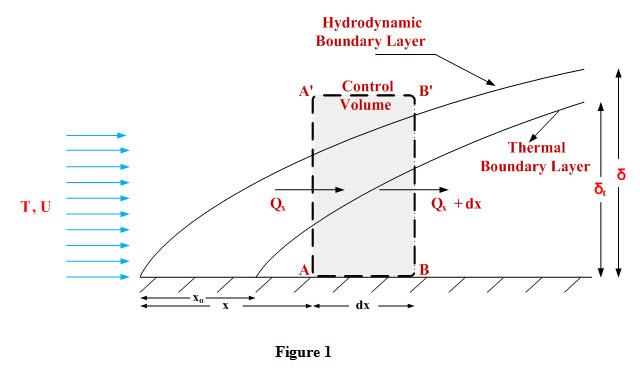
Mass of fluid entering into control volume through left face AA’

\[ = \,\int\limits_0^H {\rho \,u\,dy} \]                (1)

Mass of fluid leaving control volume through right face BB’

\[=\,\int\limits_0^H {\rho \,u\,dy} \,\, + \,\frac{\partial }{{\partial x}}\left[ {\int\limits_0^H {\rho \,u\,dy} \,} \right]dx\]             (2)

Mass of fluid entering from top face A’B’ of control volume

\[ = \,\,\frac{\partial }{{\partial x}}\left[ {\int\limits_0^H {\rho \,u\,dy} \,} \right]dx\]              (3)

Heat Influx through face AA’

\[{Q_x} = \,\,mass\, \times \,specific\,heat\, \times \,temperature\]

\[{Q_x} = \,\int\limits_0^H {\rho \,u\,dy}\times \,C\, \times \,T\]

\[ = \,\rho C\,\int\limits_0^H {\,u\,Tdy}\]                         (4)

Heat efflux through face BB’

\[{Q_{x + dx}}\, = \,\,\int\limits_0^H {\,u\,T} \,\, + \frac{\partial }{{\partial x}}\left[ {\rho C\int\limits_0^H {\,u\,Tdy} } \right]\,dx\]             (5)

The upper face A’B’ of the control volume is out of the thermal boundary layer and there temperature is constant at T_f. Therefore, energy influx is

\[{Q_h} = \,\,\frac{\partial }{{\partial x}}\left[ {\int\limits_0^H {\rho \,u\,dy} \,} \right]dx\,C\,{T_f}\]          (6)

Heat is conducted in to the lower face of the control volume at the rate.

\[{Q_c} = \, - kA{\left( {\frac{{\partial T}}{{\partial y}}} \right)_{y = 0}}\]

\[{Q_c} = \, - kdx\, \times \,1{\left( {\frac{{\partial T}}{{\partial y}}} \right)_{y = 0}}\]            (7)

An energy balance of the control volume gives:

\[\rho C\,\int\limits_0^H {\,u\,Tdy} \,\, + \frac{\partial }{{\partial x}}\left[ {\rho C\,\int\limits_0^H {\,u{T_f}\,dy} \,} \right]dx\,\, - kdx\,{\left( {\frac{{\partial T}}{{\partial y}}} \right)_{y = 0}} = \,\rho C\,\int\limits_0^H {\,u\,Tdy} \,\, + \frac{\partial }{{\partial x}}\left[ {\rho C\,\int\limits_0^H {\,uT\,dy} \,} \right]dx\]  (8)

Rearranging equation (8), we get,

\[\frac{d}{{dx}}\left[ {\,\int\limits_0^H {\,u\left( {{T_f} - T} \right)\,dy} \,} \right]\,\, = \frac{k}{{\rho C}}\,{\left( {\frac{{dT}}{{dy}}} \right)_{y = 0}}\]

\[\frac{d}{{dx}}\left[ {\,\int\limits_0^H {\,u\left( {{T_f} - T} \right)\,dy} \,} \right]\,\, = \alpha \,{\left( {\frac{{dT}}{{dy}}} \right)_{y = 0}}\]           (9)

Where α represents thermal diffusivity

Equation (9) represents the integral equation for the boundary layer for constant properties and constant free stream temperature T_f.

The net viscous work done with in the control volume is given by the equation

\[\mu \,\int\limits_0^H {\frac{{{\partial ^2}u}}{{\partial {y^2}}}} \,dxdy\]           (10)

If the net viscous work done is also considered in the energy balance, then the integral equation would become

\[\frac{d}{{dx}}\left[ {\,\int\limits_0^H {\,u\left( {{T_f} - T} \right)\,dy} \,} \right]\, + \,\frac{\mu }{{\rho C}}\int\limits_0^H {\frac{{{\partial ^2}u}}{{\partial {y^2}}}} \,dy = \frac{k}{{\rho C}}\,{\left( {\frac{{dT}}{{dy}}} \right)_{y = 0}}\]         (10)

The term related to viscous work is generally very small and is usually neglected.

To develop an expression for convective heat transfer coefficient for laminar flow over a plate, cubic velocity and temperature distribution in integral boundary layer equation will be used.

i) The temperature distribution with in the boundary layer is given as

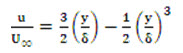
\[\frac{u}{{{u_f}}}\, = \,\frac{3}{2}\left( {\frac{y}{\delta }} \right)\, - \,\frac{1}{2}{\left( {\frac{y}{\delta }} \right)^3}\,\]       (11)

ii) Temperature distribution with in the boundary layer satisfies the conditions;

     At y = 0, T = T

     At y = δ_t,    \[\frac{{dT}}{{dy}}\, = \,0\]

    At y = δ_t, T = T_f

     At y = 0,     \[\frac{{{d^2}T}}{{d{y^2}}}\, = \,0\]

These boundary conditions have same form as those on \[\frac{u}{{{u_f}}}\,\] . Therefore, when these are fitted to a cubic polynomial

\[\frac{\theta }{{{\theta _f}}}\, = \,a\, + \,b\left( {\frac{y}{{{\delta _t}}}} \right)\, + c{\left( {\frac{y}{{{\delta _t}}}} \right)^2}\, + d{\left( {\frac{y}{{{\delta _t}}}} \right)^3}\]       (12)

Temperature distribution acquires the form

\[\frac{\theta }{{{\theta _f}}}\, = \,\frac{{T - {T_s}}}{{{T_f} - {T_s}}} = \frac{3}{2}\left( {\frac{y}{{{\delta _t}}}} \right)\, - \frac{1}{2}{\left( {\frac{y}{{{\delta _t}}}} \right)^3}\,\]       (13)

Multiplying and dividing right hand side of the integral equation by \[{u_f}\left( {{T_f} - T} \right)\] , we can write

\[\alpha \,{\left( {\frac{{dT}}{{dy}}} \right)_{y = 0}} = {u_f}\left( {{T_f} - T} \right)\frac{d}{{dx}}\left[ {\,\int\limits_0^H {\,\frac{{u\left( {{T_f} - T} \right)}}{{{u_f}\left( {{T_f} - T} \right)}}\,dy} \,} \right]\,\]

\[=\,{u_f}\left( {{T_f} - {T_s}} \right)\frac{d}{{dx}}\left[ {\,\int\limits_0^H {\,\frac{u}{{{u_f}}}\left( {1 - \frac{{\left( {T - {T_s}} \right)}}{{\left( {{T_f} - {T_s}} \right)}}} \right)\,dy} \,} \right]\]

Using equations (12) and (13), we can write

\[\alpha \,{\left( {\frac{{dT}}{{dy}}} \right)_{y = 0}}\, = \,{u_f}\left( {{T_f} - {T_s}} \right)\frac{d}{{dx}}\left[ {\,\int\limits_0^H {\,\left\{ {\frac{3}{2}\left( {\frac{y}{\delta }} \right)\, - \,\frac{1}{2}{{\left( {\frac{y}{\delta }} \right)}^3}\,} \right\}\left\{ {\frac{3}{2}\left( {\frac{y}{{{\delta _t}}}} \right)\, - \frac{1}{2}{{\left( {\frac{y}{{{\delta _t}}}} \right)}^3}\,\,} \right\}\,dy} \,} \right]\]      (14)

For most of the gases thermal boundary layer is thinner than the hydrodynamic boundary layer δ_t < δ. Therefore the upper limit of integration in equation (14) has been changed to δ_t as for y > δ_t, the integrand will become zero. Let ‘r’ represents thickness ratio and it is equal to δ_t/δ.

Upon integrating equation (14) between limits, we get

\[\alpha \,{\left( {\frac{{dT}}{{dy}}} \right)_{y = 0}}\, = \,{u_f}\left( {{T_f} - {T_s}} \right)\frac{d}{{dx}}\left[ {\delta \,\left( {\frac{3}{{20}}{r^2} - \frac{3}{{280}}{r^4}} \right)} \right]\]        (15)

As δ_t < δ, r < 1, therefore, term involving r⁴ may be neglected

\[\alpha \,{\left( {\frac{{dT}}{{dy}}} \right)_{y = 0}}\, = \,\frac{3}{{20}}{u_f}\left( {{T_f} - {T_s}} \right)\frac{d}{{dx}}\left[ {\delta {r^2}} \right]\]       (16)

Using temperature distribution equation (13), we can write

\[\frac{{T - {T_s}}}{{{T_f} - {T_s}}} = \frac{3}{2}\left( {\frac{y}{{{\delta _t}}}} \right)\, - \frac{1}{2}{\left( {\frac{y}{{{\delta _t}}}} \right)^3}\,\]

\[T\, = \,{T_s} + \left( {{T_f} - {T_s}} \right)\left[ {\frac{3}{2}\left( {\frac{y}{{{\delta _t}}}} \right)\, - \frac{1}{2}{{\left( {\frac{y}{{{\delta _t}}}} \right)}^3}} \right]\]

\[\frac{{dT}}{{dy}} = \left( {{T_f} - {T_s}} \right)\left[ {\frac{3}{{2{\delta _t}}}\, - \frac{3}{{2\delta _t^3}}{y^2}} \right]\]

\[{\left( {\frac{{dT}}{{dy}}} \right)_{y = 0}} = \frac{{3\left( {{T_f} - {T_s}} \right)}}{{2{\delta _t}}} = \frac{{3\left( {{T_f} - {T_s}} \right)}}{{2r\delta }}\]    (17)

Substituting the value of  \[{\left( {\frac{{dT}}{{dy}}} \right)_{y = 0}}\] from equation (17) in equation (16), we get

\[\frac{3}{2}\alpha \frac{{\left( {{T_f} - {T_s}} \right)}}{{r\delta }} = \frac{3}{{20}}{u_f}\left( {{T_f} - {T_s}} \right)\frac{d}{{dx}}\left[ {\delta {r^2}} \right]\]

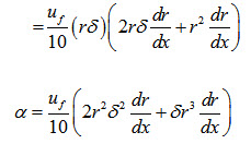
\[\alpha= \frac{{{u_f}}}{{10}}\left( {r\delta } \right)\frac{d}{{dx}}\left[ {\delta {r^2}} \right]\]

     (18)

Using the hydrodynamic boundary layer equations

\[\delta \frac{{d\delta }}{{dx}} = \frac{{140}}{{13}}\frac{v}{{{u_f}}}\,\,and\,{\delta ^2} = \frac{{280}}{{13}}\frac{{vx}}{{{u_f}}}\,\]

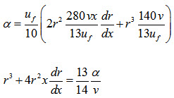
Substituting these values in equation (18), we get

(19)

Equation (19) is a linear differential equation of first order in r³ and general solution for it is given as

\[{r^3} = C\,{x^{ - \frac{3}{4}}} + \frac{{13}}{{14}}\,\frac{\alpha }{v}\]          (20)

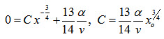
The constant C is determined by using the boundary condition

At x=x_o,  \[{r^3} = {\left( {\frac{{{\delta _t}}}{\delta }} \right)^3} = 0\]

        (21)

Substituting the value of C from equation (21) into equation (20), we get

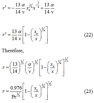
If heating of the plate starts from the leading edge of the plate, then x_o=0. Equation (23) becomes

             (24)

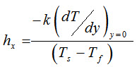
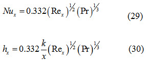
The local heat transfer coefficient can be determined as

           \[\frac{Q}{A}={h_x}\left( {{T_s} - {T_f}} \right)=- k{\left( {\frac{{dT}}{{dy}}} \right)_{y = 0}}\]

     (25)

Substituting the value of   from equation (17) in to equation (25)

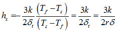        (26)

We know that

     (27)

Substituting the values of δ from equation (27) and r from equation (23) in equation (26)

 

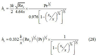
Nusselt Number can be expressed as

                                   

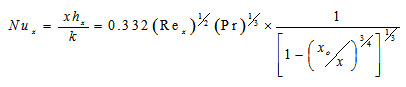
If the entire length of the plate is heated, x_o=0

 

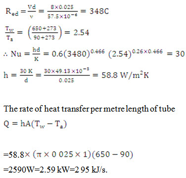
Problem 11.1  Air at atmospheric pressure and 90° C flows with a velocity of 8 m/s across a tube of 25 mm diameter. The tube is maintained at a temperature of 650° C. Calculate the rate of heat transfer per metre length of tube. Use the following relation suggested by Nusselt.

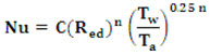
Where \[Tw\] and \[Ta\]  are the absolute temperatures of the tube surface and air.

Take C=0.6 and n = 0.466 if 40<Red <4000

Take the following properties of air at  

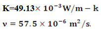
Solution:

     

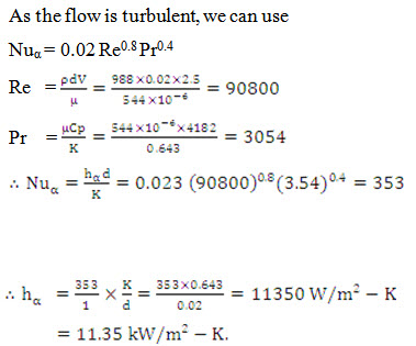
Problem 11.2  Calculate the heat transfer coefficient for water flowing through a 2 cm diameter tube with a velocity of 2.5 m/s. The average temperature of the water is 50°C and surface temperature of the tube is slightly below this temperature.

Assume the flow is turbulent.

 The properties at 50°C are given below.

C_p = 4180 J/kgK,       K = 0.643 W/mK

Solution:

                              

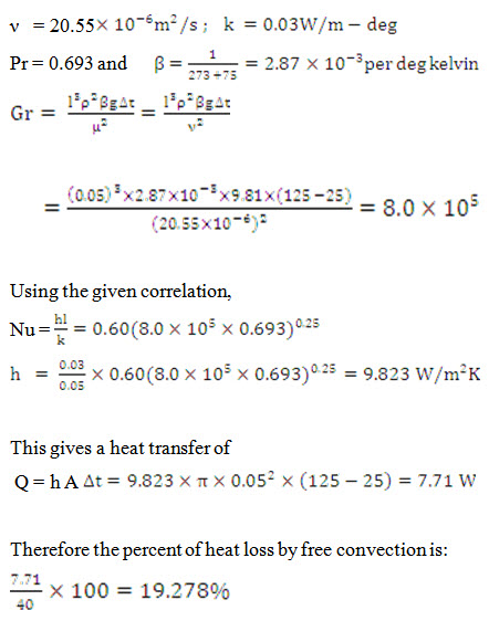
Problem 10.8  Estimate the heat transfer from a 40 W incandescent bulb at 125°C to 25°C in quiescent air. Approximate the bulb as a 50 mm diameter sphere. What percent of the power is lost by free convection?

The appropriate correlation for the convection for the convection coefficient is

           Nu = 0.60 (Gr Pr)^0.25

Where the different parameters are evaluated at the mean film temperature, and the characteristic length is the diameter of the sphere.

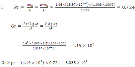
Solution:        At the mean film temperature, t_f = (125+25)/2=75°C, the thermo- physical   properties for air are:

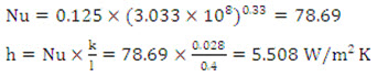
Problem 10.9  A hot square plate 40 cm  40 cm at 100°C is exposed to atmospheric air at 20°C. Make calculations for the heat loss from both surfaces of the plate, if a the plate is kept vertical (b) plate is kept horizontal.

The following empirical aorrelations have been suggested:

Nu = 0.125 (Gr Pr)^0.33 for vertical position of plate, and

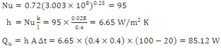
Nu = 0.72 (Gr Pr)^0.25 for upper surface

      = 0.35 (Gr Pr)^0.25 for lower surface

Where the air properties are evaluated at the mean temperature.

Solution: 

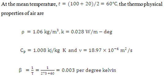
(a) When the plate is oriented vertically,

                

This gives a heat transfer of : Q = 2 h A Δt

The factor 2 accounts for two sides of the plate

(b) When the plate is positioned horizontally

(i) For upper surface:

(ii) For lower surface:

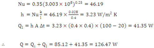
Comments: The above calculations show that the plate loses more heat when it is oriented vertically. Obviously natural cooling can be achieved more effectively by keeping the plate in vertical position.

Problem 11.3  Air at 25°C and 1 bar flows over a flat plate at a speed 1.25 m/s. Calculate the boundary layer thickness at distances of 15 cm and 30 cm from the leading edge of the plate. What would be the mass entrainment (mass flow entering the boundary layer) between these two sections? Assume parabolic velocity distribution

The velocity of air at 25°C is stated to be 6.62kg/hr m.

Solution:

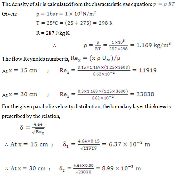
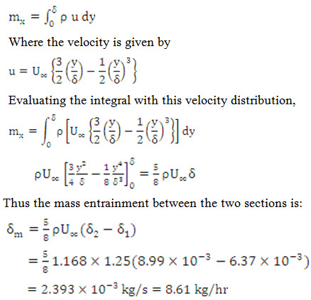
(b) At any position, the mass flow in the boundary layer is given by the integral

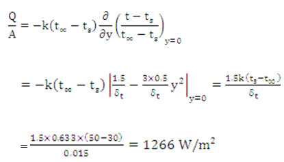
Example11.4 A small thermo-couple is positioned in a thermal boundary layer near a flat plate past which water flows at 30°C and 0.15 m/s. The plate is heated to a surface temperature of 50°C and at the location of the proble, the thickness of thermal boundary layer is 15mm. if the temperature profile as measured by the probe is well-represented by

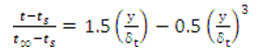
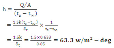
Determine (a) the heat flux from plate to water; and (b) the heat transfer coefficient

Solution:   At the mean film temperature t_f = (30+50)/2=40°C, the thermal conductivity of water is 0.633 W/m-deg.

(b) Heat transfer coefficient,

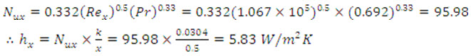
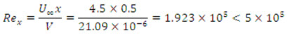
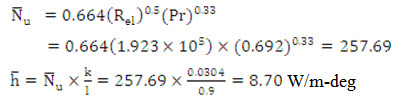
Example11.5 Air at 25°C approaches a 0.9m long by 0.6 m wide flat plate with an approach velocity 4.5 m/s. The plate is heated to a surface temperature of 135°C. Make calculations for:

a) Local heat transfer coefficient at a distance of 0.5 m from the leading edge;

b) Total rate of heat transfer from the plate to the air

Solution:  At the mean film temperature t_f = (25+135)/2=80°C, the thermo-physical properties of air are:

v = 21.0910^-6 m²/s   ;   k = 0.0304 W/m-deg  ;  p_r = 0.692

a)     

The flow is laminar at a distance of 0.5 m from the leading edge, and accordingly

b)  For the entire plate length l=0.9 m

                      Obviously the film is laminar for the entire plate length, and accordingly

Heat loss from one side of the plate,

Example11.6 Atmospheric air at 30°C temperature and free stream velocity of 2.5 m/s flows along the length of plate maintained at a uniform surface temperature of 90°C. The length, width and thickness of the plate is 100 cm, 50 cm and 2.5 cm. if thermal conductivity of the plate material is 25 W/m-deg, make calculations for (a) heat lost by the plate; (b) temperature of bottom surface of the plate for steady state conditions.

Solution:  At the mean film temperature t_f = (50+100)/2=75°C, the thermo-physical properties  of air are:

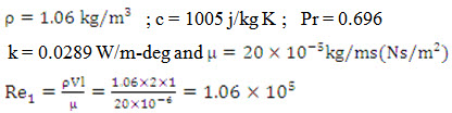
The Reynolds number is less than 510⁵, hence the flow is laminar and accordingly

Convective heat loss from the plate,

This convective heat loss must be conducted through the plate. Then from energy balance

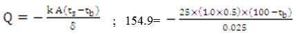
Bottom temperature of the plate,