Heat and Mass Transfer 2(2+0)

Lesson 16. Laminar Forced Flow in a Tube

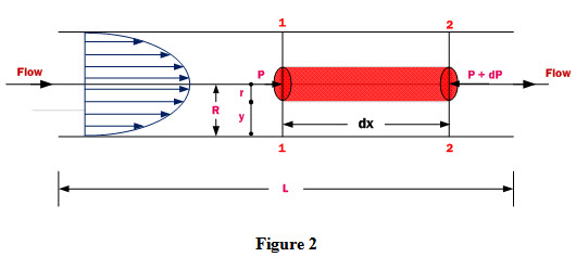
For a fully developed flow, velocity at sections 1-1 and 2-2 of the concentric cylinder is equal and pressure forces are balanced by the viscous shear forces.

Net pressure force acting on concentric cylinder

\[ = P\pi {r^2} - \left( {P + \frac{{\partial P}}{{\partial x}}dx} \right)\pi {r^2}\]       (1)

Viscous Shear force acting

\[ = 2\pi rdx\, \times \,\tau \]      (2)

Under equilibrium, net pressure force is equal to viscous shear force

\[\left( { - \frac{{\partial P}}{{\partial x}}dx} \right)\pi {r^2} = \]   \[2\pi rdx\, \times \,\tau \]      (3)

Dividing both sides of the equation (3) by volume of concentric cylinder, \[\pi {r^2}dx\]  , we get

\[\frac{{\partial P}}{{\partial x}}=- \frac{{2\tau }}{r}\]                 

Or    \[\frac{{dP}}{{dx}}=- \frac{{2\tau }}{r}\]                                                           

Or    \[\tau=-\frac{r}{2}\frac{{dP}}{{dx}}\]       (4)

Invoking Newton’s Law of viscosity for laminar flow

\[\tau= \mu \frac{{du}}{{dy}}=- \mu \frac{{du}}{{dr}}\]      (5)

  -ve sign is because ‘r’ is measured in a direction opposite to ‘y’.

Substituting the value of   from equation (4) in equation (5), we get

\[ - \frac{r}{2}\frac{{dP}}{{dx}}=- \mu \frac{{du}}{{dr}}\]            

\[\frac{{du}}{{dr}} = \frac{r}{{2\mu }}\frac{{dP}}{{dx}}\]     (6)

Integrating equation (6) twice wrt to ‘r’, we get

\[u = \frac{{{r^2}}}{{4\mu }}\frac{{dP}}{{dx}} + C\]       (7)

Applying boundary condition to equation (7)

     At r=R, u=0

\[C =- \frac{1}{{4\mu }}\frac{{dP}}{{dx}}{R^2}\]     (8)

Substituting the value of constant C in equation (7), we get

\[u = \frac{1}{{4\mu }}\left( { - \frac{{dP}}{{dx}}} \right)\left( {{R^2} - {r^2}} \right)\]          (9)

Equation (9) gives velocity distribution and location of maximum velocity can be obtained by differentiating equation (9) with respect to ‘x’ and equate it equal to zero.

\[\frac{{du}}{{dx}} = \frac{1}{{4\mu }}\left( { - \frac{{dP}}{{dx}}} \right)\left( { - 2r} \right) = 0\]        

        Or r=0

Therefore, maximum velocity occurs at centre of pipe and its value is given by

\[{u_{\max }} = \frac{1}{{4\mu }}\left( { - \frac{{dP}}{{dx}}} \right)\left( {{R^2}} \right)\]       (10)

Dividing equation (9) by equation (10), we get

\[\frac{u}{{{u_{\max }}}} = 1 - {\left( {\frac{r}{R}} \right)^2}\]           (11)

Average Velocity:

In order to determine the average velocity, volumetric flow is equated to the integrated paraboloid flow.

\[V\,\pi {R^2} = \int\limits_0^R {u\,(2\pi r)dr} \]           (12)

Substituting the value of ‘u’ from equation (11) in equation (12), we get

\[V\,\pi {R^2} = \int\limits_0^R {{u_{\max }}\,(1 - {{\left( {\frac{r}{R}} \right)}^2})2\pi rdr} \]       

\[V\,\pi {R^2} = 2\pi {u_{\max }}\int\limits_0^R {\,(r - \frac{{{r^3}}}{{{R^2}}})dr} \]

\[V\,\pi {R^2} = 2\pi {u_{\max }}\left| {\frac{{{r^2}}}{2} - \frac{{{r^4}}}{{4{R^2}}}} \right|_0^R\]

\[V\,\pi {R^2} = 2\pi {u_{\max }}\left| {\frac{{{R^2}}}{2} - \frac{{{R^4}}}{{4{R^2}}}} \right|\, = \,2\pi {u_{\max }}\frac{{{R^2}}}{4}\]

\[V\, = \,\frac{{{u_{\max }}}}{2}\]        (13)

Substituting value of ‘u_max’ from equation (10) in equation (43), we get

\[V\, = \,\frac{1}{{8\mu }}\left( { - \frac{{dP}}{{dx}}} \right)\left( {{R^2}} \right)\]        (14)

The pressure gradient dP/dx is usually is expressed in terms of friction factor and is given as

\[ - \frac{{dP}}{{dx}}\, = \,\frac{f}{d}\frac{{\rho {V^2}}}{2}\]         (15)

Where \[\frac{{\rho {V^2}}}{2}\] is the dynamic pressure of mean flow

d is the tube diameter

f is the friction factor

From equations (14) and (15), we get

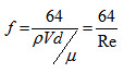           (16)

The above equation is valid for laminar flow, Re<2000

Using equation (15), pressure drop for a finite length between points x₁ and x_2, which are ‘L’ distance apart, can be expressed as

\[\frac{{{P_1} - {P_2}}}{{{x_2} - {x_1}}}\, = \,\frac{f}{d}\frac{{\rho {V^2}}}{2}\]      

\[{P_1} - {P_2} = \frac{f}{d}\frac{{\rho {V^2}}}{2}\left( {{x_2} - {x_1}} \right)\]        

\[{P_1} - {P_2} = \frac{f}{d}\frac{{\rho {V^2}}}{2}\left( L \right)\]         (17)

Substituting the value of ‘f’ from equation (16) in equation (17), we get

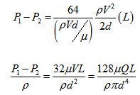       (18)

Where ‘Q’ is volumetric flow through the tube and is expressed as

Q= Velocity Ҳ Area of cross-section of the tube

    =  V Ҳ (π/4) d²

Equation (18) is known as Hagen-Poiseuille equation and represents a fully developed flow in which velocity profile dose not vary along the pipe axis.

Temperature Distribution:

In order to develop temperature distribution, let us consider flow of heat through an elementary area of length dx and thickness dr as shown in Figure 1 in which conduction along the axis is neglected.

Heat being conducted in to the element is expressed as

\[d{Q_r} =- k2\pi rdx\frac{{\partial T}}{{\partial r}}\]             (19)

Heat being conducted out of the element is expressed as

\[d{Q_{r + dr}} =- k2\pi \left( {r + dr} \right)dx\frac{\partial }{{\partial r}}\left( {T + \frac{{\partial T}}{{\partial r}}dr} \right)\]           (20)

Net heat conducted in to the element is obtained by subtracting equation (19) from equation (20) and is equal to

\[ - k2\pi rdx\frac{{\partial T}}{{\partial r}}+- k2\pi \left( {r + dr} \right)dx\left( {\frac{{\partial T}}{{\partial r}} + \frac{{{\partial ^2}T}}{{\partial {r^2}}}dr} \right)\]           (21)

Net heat convected out of the element is given as

\[d{Q_{conv}}=\rho\left( {2\pi rdr} \right)u{C_p}\frac{{\partial T}}{{\partial x}}dx\]           (22)

Under equilibrium conditions, net heat conducted in to the element is equal to the net heat convected out

\[ - k2\pi rdx\frac{{\partial T}}{{\partial r}}+ - k2\pi \left( {r + dr} \right)dx\left( {\frac{{\partial T}}{{\partial r}} + \frac{{{\partial ^2}T}}{{\partial {r^2}}}dr} \right) = \rho \left( {2\pi rdr} \right)u{C_p}\frac{{\partial T}}{{\partial x}}dx\]      (23)

Simplification and re-arrangement of equation (23) yields

\[\frac{1}{{ur}}\frac{\partial }{{\partial r}}\left( {r\frac{{\partial T}}{{\partial r}}} \right) = \frac{1}{\alpha }\frac{{\partial T}}{{\partial x}}\]             (24)

Substituting the value of velocity ‘u’ from equation (11) in equation (24), we get

\[\frac{\partial }{{\partial r}}\left( {r\frac{{\partial T}}{{\partial r}}} \right)=\frac{1}{\alpha }\frac{{\partial T}}{{\partial x}}{u_{\max }}\left( {1 - {{\left( {\frac{r}{R}} \right)}^2}} \right)r\]              (25)

Integrating equation (25) twice with respect to ‘r’, we get

\[\left( {r\frac{{\partial T}}{{\partial r}}} \right)=\frac{1}{\alpha }\frac{{\partial T}}{{\partial x}}{u_{\max }}\left( {\frac{{{r^2}}}{2} - \frac{{{r^4}}}{{4{R^2}}}} \right) + {C_1}\]

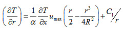            (26)

\[T = \frac{1}{\alpha }\frac{{\partial T}}{{\partial x}}{u_{\max }}\left( {\frac{{{r^2}}}{4} - \frac{{{r^4}}}{{16{R^2}}}} \right) + {C_1}{\log _e}r + {C_2}\]      (27)

Applying the boundary conditions,

At r=0, \[\left( {\frac{{\partial T}}{{\partial r}}} \right) = 0\]   and again at r=0, T=T_c, we get

C₁=0 and C₂=T_c

Substituting the values of C₁ and C₂ in equation (27), we get

\[T = \frac{1}{\alpha }\frac{{\partial T}}{{\partial x}}{u_{\max }}\left( {\frac{{{r^2}}}{4} - \frac{{{r^4}}}{{16{R^2}}}} \right) + {T_c}\]     (28)

Multiplying and dividing the right side of equation (28) by R², we get

\[T = \frac{{{u_{\max }}{R^2}}}{\alpha }\frac{{\partial T}}{{\partial x}}\left( {\frac{{{r^2}}}{{4{R^2}}} - \frac{{{r^4}}}{{16{R^4}}}} \right) + {T_c}\]

\[T - {T_c} = \frac{{{u_{\max }}{R^2}}}{{4\alpha }}\frac{{\partial T}}{{\partial x}}\left( {{{\left( {\frac{r}{R}} \right)}^2} - \frac{1}{4}{{\left( {\frac{r}{R}} \right)}^4}} \right)\]        (29)

Equation (29) represents the temperature distribution.

By using fundamental heat conduction and convection equations, heat flux coefficient can be obtained.

\[Q = hA({T_w} - {T_b}) =- kA{\left( {\frac{{\partial T}}{{\partial r}}} \right)_{r = 0}}\]        (30)

Where T_w is the wall temperature and T_b is the average bulk temperature of the fluid and mathematically it is expressed as

\[{T_b} = \frac{{\int\limits_0^R {\rho (2\pi rdr)u{C_p}T} }}{{\int\limits_0^R {\rho (2\pi rdr)u{C_p}} }}\]              (31)

For an incompressible fluid having constant density and specific heat, equation (31) can be expressed as

\[{T_b} = \frac{{\int\limits_0^R {uTrdr} }}{{\int\limits_0^R {urdr} }}\]             (32)

Generally, average value of bulk fluid temperature is used in the calculation of average heat transfer coefficient and given as

\[{T_b} = \frac{{{T_{inlet}} + {T_{outlet}}}}{2}\]

             

Combined Natural and Forced Convection

Heat transfer by Natural convection occurs in a fluid if there exists a temperature gradient with in the fluid body. Heat transfer by forced convection is always accompanied by natural convection. Since heat transfer coefficient in case of forced convection are much higher as compared to the heat transfer coefficients associated with natural convection, therefore, heat transfer by natural convection is generally neglected in case of forced convection. If velocity of fluid is high, effect of neglecting natural convection will not introduce any appreciable error, however at low velocities, the effect of ignoring natural convection may result in considerable error. Therefore, it becomes imperative to define a criterion to assess the magnitude of natural convection in forced convection.

The parameter Gr/Re² represents relative significance of natural convection to forced convection as heat transfer coefficient is function of Grashoff number, Gr in natural convection and Reynolds number, Re in forced convection.

If Gr/Re² < 0.1,  Natural convection is neglected.

If Gr/Re² > 10,   Forced convection is neglected.

If  0.1< Gr/Re²<10, Neither Natural nor forced convection is negligible. Both are to be considered.

In case when both natural and forced convection are considered, natural convection may enhance or reduce the natural convection depending upon the relative motion of buoyancy induced and forced convection currents.

In assisting flow, convectional currents set up due of density differences (natural convection) move in the same direction as the forced motion and natural convection assists the forced convection resulting in enhanced the heat transfer.

In opposing flow, convectional currents set up due of density differences (natural convection) move in the direction opposite to the forced motion and natural convection resists the forced convection resulting in decrease in heat transfer.

In transverse flow, convectional currents set up due of density differences (natural convection) move in a direction perpendicular to forced motion and results in mixing which enhances the heat transfer.

In order to determine heat transfer under combined natural and forced convection, following correlation is used.

       (33)

Nu_forced and Nu_Natural are determined from the correlations for pure forced and pure natural convection correlations. The plus sign is for assisting and transverse flow and negative sign is for opposing flows. Value of ‘n’ varies between 3 and 4.