Reservior & Farm Pond Design 3(2+1)

Lesson 2 Hydrological Aspects of Water Harvesting

Fig. 2.1 illustrates the basic factors considered in planning water harvesting interventions in the agricultural system. The meteorological parameters such as temperature, rainfall and evaporative demand of the atmosphere greatly affect the system hydrology. The likely future impacts of climate change on hydrological regimes also have to be taken into account.

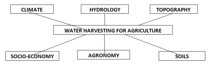
Fig. 2.1. Basic factors considered in planning water harvesting interventions. (Source: Oweis et al., 2012)

2.2 Hydrological Cycle and Water Balance

Water is available in many places and many phases above, on and below the ground surface. The transformation of water from one phase to another and its movement from one location to another in a closed system constitute the hydrological cycle. The total amount of water in the hydrosphere remains constant.

Water balances can be drawn up for a region or for an individual catchment to assess the water availability in space and time, based on which optimal water allocation policy for the agricultural production system can be established.

Fig. 2.2 shows the relationship between the various forms of water storage and water movement in a small catchment. The perceptible water in the atmosphere (W_i-W₀) is transformed and falls on the ground surface as precipitation (P) and part of it will infiltrate into the soil (F), while the other part may find its way as overland flow (Q₀) into the channels networks. Water is transferred from the land and plant surfaces to the atmosphere by evaporation (E) or through vegetation by means of transpiration (T).

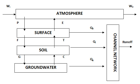
Fig. 2.2. Small catchment-scale relationship between various forms of water and its movement. (Source: Oweiset al., 2012)

If rainfall intensity exceeds the infiltration rate of soil or if the upper most parts of the soil matrix are saturated, rainwater will be collected in puddles and then overland flow occurs on the land surface as surface runoff. A portion of runoff may infiltrate into the ground or may evaporate returning to the atmosphere.

During and following precipitation soil moisture in the unsaturated subsurface zone is replenished by the process of infiltration. Once the upper soil layers are largely saturated, water will percolate down to the deeper layers, recharging the groundwater (G). Some will also flow laterally through the soil (Q_i), known as interflow, into the channel network and contributes to stream flow during dry periods. During prolonged dry periods, soil moisture may be replenished through capillary contribution (C) from shallow groundwater table. Overland flow, interflow and groundwater contribution (Q_g) are all combined and modified in the channel or river network to form the runoff from the catchment.

Hydrological modeling tool in small watersheds may be used to assess the amount of water available for agricultural purposes. Irrigation water that infiltrates into the soil first enters the crop root zone. This water may return back to the atmosphere through evapotranspiration. This upper root-zone can hold a limited quantity of water, depending on the field capacity of soil (the amount of water that a soil retains after drainage under gravity). If water is added further to the zone when it is at field capacity, the water percolates down to the saturated or groundwater zone. Water leaves the ground water zone by capillary action into the root zone or by seepage into streams.

2.3 Hydrological Characteristics

The hydrological characteristics of a region are determined largely by its climate, topography, soil and geology. Key climatic factors are the depth, intensity and frequency of rainfall and the effects of temperature and humidity on evapotranspiration.

2.3.1 Evapotranspiration

Evaporation and transpiration are decisive elements in the design of a water harvesting system. Precipitation deposited on vegetation eventually evaporates and quantity of water reaching the soil surface is correspondingly less. Evaporation and transpiration are indicative of changes in the moisture level of a basin. Estimates of these factors are also used in determining water supply requirements of proposed irrigation projects. Consumptive water use is the total actual evapotranspiration from an area plus the water used directly in building plant tissue. Evapotranspiration is strongly related to the density of plant coverage and its stages of development. There are numerous approaches to estimate actual and potential evapotranspiration, including the water budget and lysimeter methods, but none of them is generally applicable for all purposes. In some hydrologic studies, mean basin evapotranspiration is required while in other cases we are interested to know dynamics of water needs of a particular crop cover.

2.3.2 Precipitation

Precipitation results from condensation of moisture in the atmosphere. The term denotes all forms of water that reach the earth from the atmosphere. The usual forms are rainfall, snowfall, hail, frost and dew. Of all these, only the first two contribute significant amount of water. Rainfall is the predominant form of precipitation causing stream flow. The following are key terms used for rainfall analysis.

• Rainfall intensity is the quantity of rain falling in a given time over an area and can be expressed in terms of cm/h or mm/h

• Rainfall duration is the time during which a rainfall event takes place.

• Frequency of a rainfall is the frequency with which a given amount of rain occurs over a given period, for example, once in four year or once in six year, etc.

• Magnitude of rainfall is the total amount of rain falling at a point over a given period of time, i.e. daily, monthly, annually.

2.3.3 Frequency Analysis and Design Rainfall

Frequency analysis can be used to estimate the frequency of occurrence of past events, on the probability of occurrence of future events. Rainfall is a continuous random variable, varying with time (stochastic variable) and can take any value greater than or equal to zero. Exceedance probability is the probability that the rainfall will be greater than or equal to a given value. For example, if the exceedance probability of 300 mm annual rainfall for a given location is 20%, one can expect that on an average the occurrence of annual rainfall equal or exceeds 300mm is one in five years.

The return period or recurrence interval is the average time between occurrences of an event with a certain magnitude or greater. The return period T is related to exceedance probability, P_eas follows;

P_e=1/T                                           (2.1)

Thus, for example, if the exceedance probability of a 250 mm annual rainfall for an area is 67%, the annual rainfall may equal or exceed 250 mm twice in a three year period.

For water harvesting purposes, frequency analysis is usually performed for annual and monthly rainfall data. Frequency analysis is made by plotting rainfall amounts against their cumulative probability, P_c. The relationship between P_e and P_c is:

P_e =1- P_c                                         (2.2)

For example, the P_e of zero annual rainfall in any location is 100%, therefore, P_c=0.

Plotting rainfall against P_e or P_c can be done in various ways. For water harvesting, it is sufficient to use the Weibull plotting position formula, because the required design value for rainfall lies within the range of the data. The Weibull formula is:

P_e= m/(N+1)                                              (2.3)

Where, m = rank of the event, m=1 for the largest value, and N = number of rainfall events or sample size.

For example, Table 2.1 presents the annual rainfall for 22 years ranked in descending order and its third column contains the exceedance probability based on Eqn. 2.3.

The design rainfall is the amount of rainfall that is expected to be equaled or exceeded at a selected level of dependability. In Table 2.1, the design annual rainfall at a 70% exceedance probability or dependability is 155 mm. This means that annual rainfall is expected to be 155 mm or more in 7 years out of 10. Similarly, design monthly or weekly rainfall can be evaluated. Usually 67% probability of exceedance is taken for the design of agricultural water harvesting systems.

Table  2.1. Frequency analysis of annual rainfall using Weibull plotting

                   Position method (Source: Oweiset al., 2012)

Rainfall (mm)	Rank (m)	Pe (%)
399	1	4
387	2	9
335	3	13
315	4	17
293	5	22
291	6	26
249	7	30
244	8	35
238	9	39
235	10	43
223	11	48
213	12	52
194	13	57
182	14	61
174	15	65
155	16	70
154	17	74
150	18	78
109	19	83
106	20	87
98	21	91
93	22	96

2.4 Factors Affecting Runoff

Surface runoff is affected by many interrelated factors, such as soil properties, rainfall characteristics (intensity, duration and frequency),and catchment characteristics (land cover, slope, size and shape).

2.4.1 Soil Properties

Coarse textured soils have stable structures and exhibit high infiltration rates, thus resulting in little or no runoff. Fine textured soils swell when wetted and shrink and crack upon drying. Infiltration rate is high initially but falls rapidly to very low level as the soil as wetted. Soil containing around 20% clay is highly prone to surface sealing, resulting in crust or cap that makes the soil surface almost impervious. It is very important to take all these soil factors into consideration when planning and designing a water harvesting system.

2.4.2 Rainfall Characteristics

Intensity, duration and frequency are the most important characteristics of rainfall for water harvesting. In general, in India the runoff producing storms are usually of high intensity and short duration. The kinetic energy of falling drops is proportional to rainfall intensity. High intensity rainfall breaks down soil aggregates at the soil surface, filling pores with fine particles. As a result, soil surface sealing develops which reduces infiltration and induces runoff. Therefore, runoff coefficients from intense short-duration rainstorms are usually greater than those from less intense rainstorms having the same depth of rainfall.

2.4.3 Catchment Characteristics

Surface roughness and vegetation impede overland flow and increase surface storage capacity. Vegetative cover also protects the soil surface against erosion and from the destructive impact of falling raindrops. This reduces the development of crusting and soil surface sealing and hence reduces runoff.

Generally, surface runoff increases with the rise in land slope angle. This is mainly because less water is retained on the soil surface and it flows more quickly towards the outlet with minimum loss by evaporation and infiltration in the catchment. Ground relief may take all kinds of shapes and sizes which affects the runoff generation.

The runoff coefficient generally decreases with the increase in catchment size and/or slope length. In water harvesting system, rainfall induces surface runoff in preferably bare, crusted and smooth land surfaces. At the lower end of the slope, runoff water is collected in shallow depressions, which also receive direct rainfall.

For macro-catchment, the rainfall-runoff process is extremely complex due to the large spatial variations in soil type, topography, and use and land cover conditions over the vast area of the runoff producing catchment. Therefore, it is important to monitor the response of the macro-catchment to major rainstorm events by measuring the runoff at carefully selected gauging stations along the flow path of runoff.

While the rainfall is infiltrating and runoff is being collected in the target area, some water will evaporate from the open water surface, but the major portion infiltrates and is stored in the root zone.

2.5 Runoff  Models Suitable for Water Harvesting

Rainfall-runoff models aim to describe surface runoff as a function of rainfall. Model parameters are calibrated to a specific location and field conditions. Here, various methods are presented to establish the relationship between rainfall and runoff for micro- and macro-catchments.

2.5.1 Micro-Catchment

Fig. 2.3 shows the response of a soil system under three different rainstorms. Storms 1 do not saturate the soil surface because the intensity is less than the saturated hydraulic conductivity of the soil, P. The storm 2 also does not produce runoff because the duration-intensity that exceeded P was relatively short. Storm 3, however, saturates the soil surface by time t_s, satisfies the surface storage and generates surface runoff. Surface runoff has started at t_r and ended at t_e (Fig. 2.3). A curve for cumulative runoff is also shown. Between t_s and t_r, the surface storage capacity (SSC) has been filled.

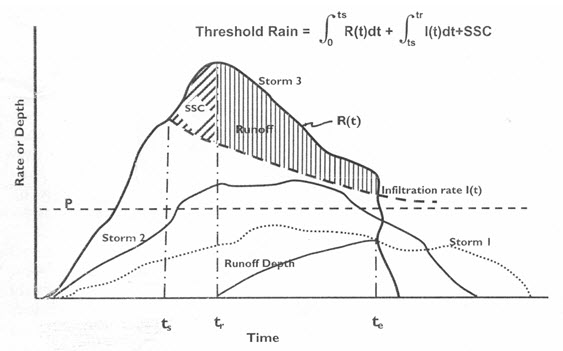
Fig. 2.3. Micro-catchment response under three different rainstorms.

(Source: Oweiset al., 2012)

Threshold rain (TR) is defined as the total rainfall depth measured from the onset of the rainstorm until the start of surface runoff flow. TR is calculated using the following equation;

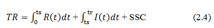
Where, t_s= time at which the soil surface becomes saturated, t_{r =} time at which runoff starts, R(t)= rainfall intensity rate, function of time t, I(t)=water infiltration rate, function time t, and SSC= surface storage capacity.

Fig. 2.4 shows one way to partition the rainwater in a micro-catchment into many components, based on a steady (constant intensity, R) rainstorm of duration T. Components 1,2 and 3 are, respectively, the first, second, and third terms in the right hand site of Eqn. 2.4. Component 4 represents the amount of excess rainwater at any point in the micro-catchment. Component 5 represent infiltration, during rain, between t_r and T. Since the distance traveled by runoff in the micro-catchment of water harvesting is small and thus negligible, no allowance is made for routing surface runoff flow. Therefore, excess rainwater at all points in the micro-catchment is summed and taken as the generated runoff. Component 3 represents surface storage, which will eventually infiltrate into the soil when the rain ceases or when the rain intensity becomes less than the infiltration capacity of the soil. Therefore, infiltration plays the major role in determining the amount of surface runoff.

There are many models (empirical, physical and numerical) to describe the behavior of the system. However, factors affecting this system and its outcome, particularly antecedent soil moisture content, soil cover and soil structure, are continuously changing during the growing season. Very few data on rainfall intensity and duration are available especially in dry areas. Furthermore, it is extremely difficult, if not impossible, to predict the intensity and duration of future rainstorms. Therefore, the only rational way to estimate surface runoff for water harvesting purposes is based on the depth of rainfall (daily, monthly or yearly).

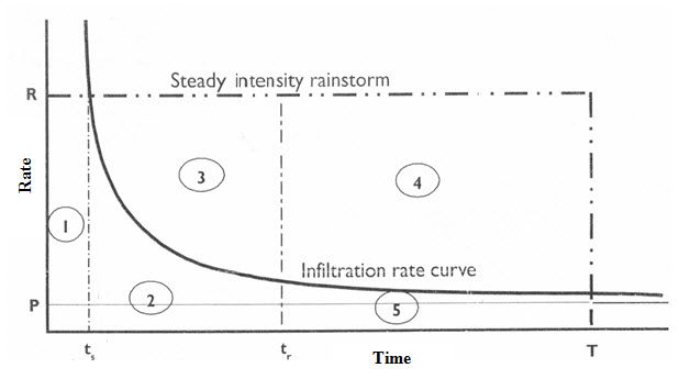
Fig. 2.4. Component of partitioning a steady intensity rainstorm of duration T for water harvesting purposes. (Source: Oweis et al., 2012)

Threshold rain is the sum of components 1, 2 and 3; component 3 and 4 (above the curve) are the surface storage and surface runoff, respectively; and component 5 is the infiltration amount between t_r and T and P is the saturated hydraulic conductivity of the soil.

The runoff coefficient is defined as the ratio of the amount of runoff to the amount of rainfall. For a single storm, the runoff coefficient (RC) can be expressed as (Fig. 2.4):

RC= component 4/rainstorm depth                      (2.5)

 

The rainstorm depth can be expressed as:

 

Rainstorm depth=TR+ Component 4+ Component 5      (2.6)

 

Equations 2.5 and 2.6 are combined and rearranged as:

 

RC=1-[(TR+ Component5)/rainstorm depth]               (2.7)

By selecting a reasonable value for TR and assuming component 5 is very small     (»zero), one can get a maximum limiting value for RC in a given area. For example, if the depth of the rainstorm in Fig. 2.4 is 10 mm and TR is taken as 4 mm, then the maximum value for RC is 0.60.

Daily rainfall represents the sum of all rainstorms during the 24 hours of the day. However, for the purposes of the present analysis, the rainstorm depth in Eqns. (2.5) and (2.7) will be taken as the daily rainfall.

In small catchments, most of runoff is in the form of sheet flow, and hence runoff plots under controlled conditions may be used to measure runoff under rainfall of differing intensities. The plot must be representative for the area to be developed for water harvesting. It is advisable to experiment on plots of various sizes (slope length and slope angles).

Overestimation of RC may result in reduced crop yields or crop failure due to water shortages. Underestimation of RC results in setting aside more land than necessary as catchment areas and endangering the safety of the water harvesting system structures. The effect of excess or deficit moisture condition varies according to the crop. Millet, for example, can tolerate drought but not waterlogging but maize does not tolerate either.

2.5.2 Macro-Catchment

Methods suitable for estimation of runoff in macro-catchments include the unit hydrograph, the soil conservation Service (SCS) curve number, and the rainfall excess model. The first two methods are relatively simple, standard, well document and can be found in most of the textbooks on hydrology and water resources systems engineering. The third method is not well known as it is more complex. A brief description of the first two methods is given below.

Unit Hydrograph Method

The unit hydrograph method is still frequently used to determine runoff, despite many limiting factors. A hydrograph is a graph of discharge passing through a particular point on a stream, plotted as a function of time. A unit hydrograph is a graph of the direct runoff of 1 mm of effective rainfall distributed uniformly over the basin area (catchment) at a uniform rate during a storm, of particular duration. Figure 2.5 shows a typical 6-hour unit hydrograph. The unit hydrograph is assumed to be representative of the runoff process for a watershed. The method is based on following three postulates:

• Constant duration of flow for a given drainage basin; the duration of flow depends on the duration of rainfall and not on its intensity.

• Linearity for rain of equal duration but of different intensity; runoff is proportional to the rainfall intensity.

• Runoff caused by several periods of rainfall can be superimposed.

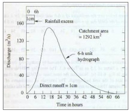
Fig. 2.5. Typical 6-h unit hydrograph.

(Source: http://static5.theconstructor.org/wp-content/uploads/2010/10/clip_ image0022.jpg)

The unit hydrograph should be derived from as many peak flows as possible. Monthly and annual mean or total flow is used to display the record of past runoff at a station.

One limitation of the unit hydrograph method is the assumption that storms occur with uniform intensity over the entire drainage basin. A unit hydrograph derived from a single storm may not be representative and it is, therefore, desirable to average unit hydrographs from several storms of about same duration.

SCS Curve Number Method

The US Soil Conservation Service (SCS) developed the curve number to estimate the effect of land treatment and land use changes upon runoff. It has been widely accepted and used for planning and design of soil and water conservation interventions. The popularity of this method is due to its simplicity, predictability, stability and its responsiveness to watershed properties affecting runoff. The parameters used in this method are to quantify physical processes although they may not be directly measurable. They usually represent spatially averaged catchment characteristics, such as surface cover type and conditions, soil type and others. An important feature of the curve number method is that the proportion of rainfall converted into runoff(runoff coefficient) increases with the rainfall depth.

Derivation of Empirical Relationships

When the data of accumulated rainfall and runoff for long-duration, high-intensity rainfalls over small drainage basins are plotted, they show that runoff only starts after some rainfall has accumulated, and that the curves asymptotically approach a straight line with a 45-degree slope. The Curve Number Method is based on these two phenomena. The initial accumulation of rainfall represents interception, depression storage, and infiltration before the start of runoff and is called initial abstraction. After runoff has started, some of the additional rainfall is lost, mainly in the form of infiltration; this is called actual retention. With increasing rainfall, the actual retention also increases up to some maximum value: the potential maximum retention.  To describe these curves mathematically, SCS method assumed that the ratio of actual retention to potential maximum retention was equal to the ratio of actual runoff to potential maximum runoff, the latter being rainfall minus initial abstraction. In mathematical form, this empirical relationship is,

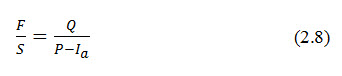
Where, F = actual retention (mm), S = potential maximum retention (mm), Q = accumulated runoff depth (mm), P = accumulated rainfall depth (mm),and I_a = initial abstraction (mm).

After runoff has started, all additional rainfall becomes either runoff or actual retention (difference between rainfall minus initial abstraction and runoff).

F = P - I_a- Q                                        (2.9)

Combining Eqn. (2.8) and (2.9),

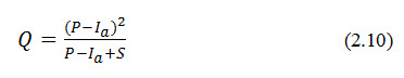
I_a assumed to be function of S as, I_a= 0.2S, then

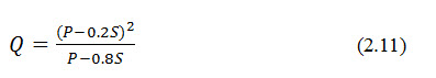
Knowing P and S, the value of Q can be calculated. Q has the same unit as that of P and is usually expressed in mm.

The curve number as defined by U.S. SCS is given by,

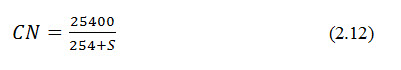
Table 2.2 presents curve numbers for various land use and hydrologic soil group. Knowing the curve number, the value of recharge capacity S is calculated (Eqn. 2.12) and using this value, the runoff Q can be estimated (Eqn. 2.11).

Hydrological Soil Group

Soil properties greatly influence the amount of runoff. In the SCS method, these properties are represented by a hydrological parameter: the minimum rate of infiltration obtained for a bare soil after prolonged wetting. The influence of both the soil’s surface condition (infiltration rate) and its horizon (transmission rate) are thereby included. This parameter, which indicates a soil’s runoff potential, is the qualitative basis of the classification of all soils into four groups. The Hydrological Soil Groups, as defined by the SCS soil scientists, are:

Group A: Soils having high infiltration rates even when thoroughly wetted and a high rate of water transmission. Examples are: deep, well to excessively drained sands or gravels.

Group B: Soils having moderate infiltration rates when thoroughly wetted and a moderate rate of water transmission. Examples are: moderately deep to deep, moderately well to well drained soils with moderately fine to moderately coarse textures.

Group C: Soils having low infiltration rates when thoroughly wetted and a low rate of water transmission. Examples are: soils with a layer that impedes the downward movement of water or soils of moderately fine to fine texture.

Group D: Soils having very low infiltration rates when thoroughly wetted and a very low rate of water transmission. Examples are: clay soils with a high swelling potential, soils with a permanently high water table, soils with a clay pan or clay layer at or near the surface, or shallow soils over nearly impervious  material.

Antecedent Moisture Condition

The soil moisture condition in the drainage basin before runoff occurs is another important factor influencing the final CN value. In the Curve Number Method, the soil moisture condition is classified in three Antecedent Moisture Condition (AMC) classes:

AMC I:  The soils in the drainage basin are practically dry (i.e. the soil moisture content is at wilting point). 

AMC II:  Average condition.

AMC III: The soils in the drainage basins are practically saturated from antecedent rainfalls (soil moisture content is at field capacity).

These classes are based on 5-day antecedent rainfall (i.e. the accumulated total rainfall preceding the runoff under consideration). In the original SCS method, a distinction was made between the dormant and the growing season to allow for differences in evapotranspiration.

Table 2.2.  Curve numbers for hydrologic soil cover complexes.

(Source: http://www.oasification.com/tablasden_en.htm)

Land use	Treatment	Hydrologic condition	Soil type
			A	B	C	D
Fallow land	Naked	-	77	86	91	94
	CR	Poor	76	85	90	93
	CR	Good	74	83	88	90
Row crops (aligned cultivated soils)	R	Poor	72	81	88	91
	R	Good	67	78	85	89
	R + CR	Poor	71	80	87	90
	R + CR	Good	64	75	82	85
	C	Poor	70	79	84	88
	C	Good	65	75	82	86
	C + CR	Poor	69	78	83	87
	C + CR	Good	64	74	81	85
	C + T	Poor	66	74	80	82
	C + T	Good	62	71	78	81
	C + T + CR	Poor	65	73	79	81
	C + T + CR	Good	61	70	77	80
Small grain (non aligned cultivated soils)	R	Poor	65	76	84	88
	R	Good	63	75	83	87
	R + CR	Poor	64	75	83	86
	R + CR	Good	60	72	80	84
	C	Poor	63	74	82	85
	C	Good	61	73	81	84
	C + CR	Poor	62	73	81	84
	C + CR	Good	60	72	80	83
	C + T	Poor	61	72	79	82
	C + T	Good	59	70	78	81
	C + T + CR	Poor	60	71	78	81
	C + T + CR	Poor	58	69	77	80
Dense leguminous crops or meadows in rotation	R	Poor	66	77	85	89
	R	Good	58	72	81	85
	C	Poor	64	75	83	85
	C	Good	55	69	78	83
	C + T	Poor	63	73	80	83
	C + T	Good	51	67	76	80
Natural pastures	-	Poor	68	79	86	89
	-	Fair	49	69	79	84
	-	Good	39	61	74	80
Pastures	C	Poor	47	67	81	88
	C	Fair	25	59	75	83
	C	Good	6	35	70	79
Permanent meadows (protected from grazing)	-	-	30	58	71	78
Brush-grassland, with brush dominating	-	Poor	48	67	77	83
	-	Fair	35	56	70	77
	-	Good	≤30	48	65	73
Mixture of woods and grassland, woody agriculture crops	-	Poor	57	73	82	86
	-	Fair	43	65	76	82
	-	Good	32	58	72	79
Woods with pastures (silvopastoral use)	-	Poor	45	66	77	83
	-	Fair	36	60	73	79
	-	Good	25	55	70	77
Woods	-	Very poor	56	75	86	91
	-	Poor	46	68	78	84
	-	Fair	36	60	70	76
	-	Good	26	52	63	69
	-	Very good	15	44	54	61
Country houses	-	-	59	74	82	86
Gravel roads	-	-	72	82	87	89
Asphalt roads	-	-	74	84	90	92

Abbreviations meaning: CR=with vegetal residue cover that extends for at least 5% of the soil surface all over the year; R=when soil labours (ploughing, sowing, etc.) are made in straight line, without considering the slope; C=when cultivation is made according to contour lines; and T=in terraces cultivations (open terraces with drainage for soil conservation)

Key words: Hydrology, Water harvesting, Catchment

References

• Owesis, T. Y., Prinz, D. and Hachum, A. Y. (2012). Rainwater Harvesting  for Agricultural in the Dry Areas. CRC Press, First Edition, pp. 11-26.

• Subramanya, K. (2009). Engineering Hydrology. Tata McGraw Hill, Third Edition, pp.155-163.

Suggested Readings

• Murthy, V.V.N. and Jha, M. K. Jha. (2011). Land and Water Management Engineering, Kalyani Publication.