Electrical M/C’s and Power Utilization 3(2+1)

LESSON 7. Transformer EMF equation and phase diagram on load

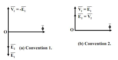
Fig. 4.1 No load phasor diagram following two conventions.

In convention 1, phasors  E1 and  E2 are drawn 180° out of phase with respect to V1   in order to convey that the respective power flow directions of these two are opposite. The second convention results from the fact that the quantities v1(t), e1(t) and e2(t) vary in unison then why not show them as co-phasal and keep remember the power flow business in one’s mind. Also remember vanishingly small magnetizing current is drawn from the supply creating the flux and in time phase with the flux.

Transformer under loaded condition

In this lesson, we shall study the behavior of the transformer when loaded. A transformer gets loaded when we try to draw power from the secondary. In practice loading can be imposed on a transformer by connecting impedance across its secondary coil. It will be explained how the primary reacts when the secondary is loaded. It will be shown that any attempt to draw current/power from the secondary, is immediately responded by the primary winding by drawing extra current/power from the source. We shall also see that mmf balance will be maintained whenever both the windings carry currents. Together with the mmf balance equation and voltage ratio equation, invariance of Volt-Ampere (VA or KVA) irrespective of the sides will be established.

We have seen that the secondary winding becomes a seat of emf and ready to deliver power to a load if connected across it when primary is energized. Under no load condition, power drawn is zero as current drawn is zero for ideal transformer. However when loaded, the secondary will deliver power to the load and same amount of power must be sucked in by the primary from the source in order to maintain power balance. We expect the primary current to flow now. Here we shall examine in somewhat detail the mechanism of drawing extra current by the primary when the secondary is loaded. For a fruitful discussion on it let us quickly review the dot convention in mutually coupled coils.

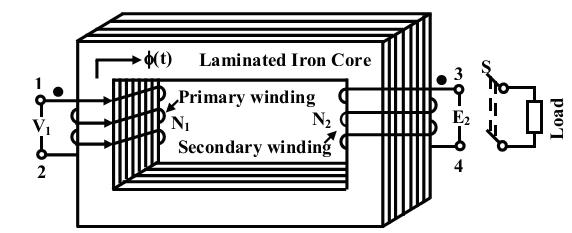
Fig. 4.2 Typical transformer

Dot convention

The primary of the transformer is energized from a.c source and potential of terminal 1 with respect to terminal 2 is v12 = Vmaxsinωt. Naturally polarity of 1 is sometimes +ve and some other time it is –ve. The dot convention helps us to determine the polarity of the induced voltage in the secondary coil marked with terminals 3 and 4. Suppose at some time t, we find that terminal 1 is +ve and it is increasing with respect to terminal 2. At that time what should be the status of the induced voltage polarity in the secondary – whether terminal 3 is +ve or –ve? If possible let us assume terminal 3 is –ve and terminal 4 is positive. If that be current the secondary will try to deliver current to a load such that current comes out from terminal 4 and enters terminal 3. Secondary winding therefore, produces flux in the core in the same direction as that of the flux produced by the primary. So core flux gets strengthened in inducing more voltage. This is contrary to the dictate of Lenz’s law which says that the polarity of the induced voltage in a coil should be such that it will try to oppose the cause for which it is due. Hence terminal 3 can not be –ve.

If terminal 3 is +ve, then we find that secondary will drive current through the load leaving from terminal 3 and entering through terminal 4. Therefore flux produced by the secondary clearly opposes the primary flux fulfilling the condition set by Lenz’s law. Thus when terminal 1 is +ve, terminal 3 of the secondary too has to be positive. In mutually coupled coils dots are put at the appropriate terminals of the primary and secondary merely to indicative the status of polarities of the voltages. Dot terminals will have at any point of time identical polarities. In the transformer of figure 4.2, it is appropriate to put dot markings on terminal 1 of primary and terminal 3 of secondary. It is to be noted that if the sense of the windings are known (as in figure 4.2), then one can ascertain with confidence where to place the dot markings without doing any testing whatsoever. In practice however, only a pair of primary terminals and a pair of secondary terminals are available to the user and the sense of the winding can not be ascertained at all. In such cases the dots can be found out by doing some simple tests such as polarity test or d.c kick test.

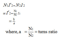
If the transformer is loaded by closing the switch S, current will be delivered to the load from terminal 3 and back to 4. Since the secondary winding carries current it produces flux in the anti clock wise direction in the core and tries to reduce the original flux. However, KVL in the primary demands that core flux should remain constant no matter whether the transformer is loaded or not. Such a requirement can only be met if the primary draws a definite amount of extra current in order to nullify the effect of the mmf produced by the secondary. Let it be clearly understood that net mmf acting in the core is given by: mmf due to vanishingly small magnetizing current + mmf due to secondary current + mmf due to additional primary current. But the last two terms must add to zero in order to keep the flux constant and net mmf eventually be once again be due to vanishingly small magnetizing current. If I2 is the magnitude of the secondary currents I2 and I2’ is the additional current drawn by the primary and then following relation must hold good.

To draw the phasor diagram under load condition, let us assume the power factor angle of the load to be θ2, lagging. Therefore the load current phasor I2  , can be drawn lagging the secondary terminal voltage E2 by θ2 as shown in the figure 4.3 as per the convention 2.

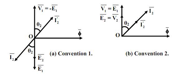
Fig. 4.3. Phasor diagram under load

At this stage, let it be suggested to follow one convention only and we select convention 2 for that purpose. Now,

Volt-Ampere delivered to the load = V2I2  = E2I2

 

Thus we note that for an ideal transformer the output VA is same as the input VA and also the power is drawn at the same power factor as that of the load.