Site pages
Current course
Participants
General
MODULE 1. Introduction to mechanics of tillage tools
MODULE 2. Engineering properties of soil, principl...
MODULE 3. Design of tillage tools, principles of s...
MODULE 4. Deign equation, Force analysis
MODULE 5. Application of dimensional analysis in s...
Module 6. Introduction to traction and mechanics, ...
Module 7. Traction model, traction improvement, tr...
Module 8.Soil compaction and plant growth, variabi...
LESSON 7. ASSESSMENT OF THE DYNAMIC PROPERTIES OF SOILS
7.1. INTRODUCTION
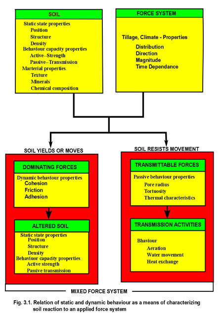
Dynamic properties are capable of characterizing soil as it reacts to applied forces. Interrelations between applied forces, dynamic properties, and behavior are implied in figure 3.1. The figure also suggests the qualitative nature of these relations. The soil and the applied forces are both of importance so that once a specific soil is isolated and a specific system of forces applied, the resulting behavior is determined. The behavior must, be considered in a restricted form ; hence, a statistical form of result is not produced. The soil and forces thus are primaryand basic, and the behavior is derived from these basic factors.
Dynamic parameters provide a means for numerically representing dynamic properties. The parameter is defined as a quantity or constant whose value varies with the soil conditions or circumstances. Each equation that defines a dynamic property contains one or more mathematical parameters that are measures of the dynamic property. Thus, for a given circumstance (soil in a specific condition), the numerical value of the parameter is a constant; but, as the soil condition varies because of such things as a change in moisture content, the numerical value of the parameter may also vary. In other words, the dynamic parameters are precisely determined by the physical properties of the soil although the exact relation may not be known. A complete quantitative description of behavior of the soil to forces can be determined after one has identified, qualitatively defined, and finally quantitatively assessed dynamic parameters of soil.
7.2. MEASURING INDEPENDENT PARAMETERS
By using appropriate apparatus, specific independent dynamic parameters of shear, tension, compression, plastic flow, friction, and adhesion can be measured under highly controlled conditions. The methods that have been developed are not completely accurate or satisfactory. Undoubtedly, these measurement techniques will be modified or improved as research is continued; however, techniques for a number of measurements have been standardized to some extent and an effort should be made to use these when practicable.
7.2.1. SHEAR STRENGTH DETERMINATION
Soils consist of individual particles that can slide and roll relative to one another. Shear strength of a soil is equal to the maximum value of shear stress that can be mobilized within a soil mass without failure taking place. The shear strength of a soil is a function of the stresses applied to it as well as the manner in which these stresses are applied. A knowledge of shear strength of soils is necessary to determine the bearing capacity of foundations, the lateral pressure exerted on retaining walls, and the stability of slopes.
A. Laboratory Methods of Shear Strength Determination
Direct shear test and the triaxial test are the two most widely used methods for determining soil shear strength. The purpose of these tests is to determine the value of cohesion (c) and angle of internal friction (f) needed in Equation 2.10 to define the soil shear failure envelope.
i. Direct Shear Test
The test is carried out on a soil sample confined in a metal box of square cross-section which is split horizontally at mid-height. A small clearance is maintained between the two halves of the box. The soil is sheared along a predetermined plane by moving the top half of the box relative to the bottom half. The box is usually square in plan of size 60 mm x 60 mm. A typical shear box is shown in figure 3.2
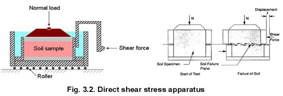
If the soil sample is fully or partially saturated, perforated metal plates and porous stones are placed below and above the sample to allow free drainage. If the sample is dry, solid metal plates are used. A load normal to the plane of shearing can be applied to the soil sample through the lid of the box.
Tests on sands and gravels can be performed quickly, and are usually performed dry as it is found that water does not significantly affect the drained strength. For clays, the rate of shearing must be chosen to prevent excess pore pressures building up. As a vertical normal load is applied to the sample, shear stress is gradually applied horizontally, by causing the two halves of the box to move relative to each other. The shear load is measured together with the corresponding shear displacement. The change of thickness of the sample is also measured. A number of samples of the soil are tested each under different vertical loads and the value of shear stress at failure is plotted against the normal stress for each test. Provided there is no excess pore water pressure in the soil, the total and effective stresses will be identical. From the stresses at failure, the failure envelope can be obtained.
Advantages of direct shear test
It is easy to test sands and gravels.
Large samples can be tested in large shear boxes, as small samples can give misleading results due to imperfections such as fractures and fissures, or may not be truly representative.
- Samples can be sheared along predetermined planes, when the shear strength along fissures or other selected planes are needed.
Disadvantages of direct shear test
The failure plane is always horizontal in the test, and this may not be the weakest plane in the sample. Failure of the soil occurs progressively from the edges towards the centre of the sample.
There is no provision for measuring pore water pressure in the shear box and so it is not possible to determine effective stresses from undrained tests.
The shear box apparatus cannot give reliable undrained strengths because it is impossible to prevent localised drainage away from the shear plane.
ii. Triaxial Test
Triaxial test.
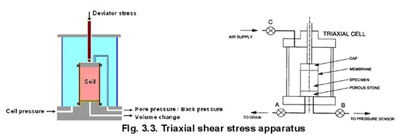
The triaxial test is carried out in a cell on a cylindrical soil sample having a length to diameter ratio of 2. The usual sizes are 76 mm x 38 mm and 100 mm x 50 mm. Three principal stresses are applied to the soil sample, out of which two are applied water/air pressure inside the confining cell and are equal. The third principal stress is applied by a loading ram through the top of the cell and is different to the other two principal stresses. A typical triaxial cell is shown in figure 3.3.
Consider a cylindrical soil sample subjected to a hydrostatic stress σ3 as shown in Figure 3.4(a) and then an additional normal stress called the deviator stress (σ′) as shown in Figure 3.4(b).
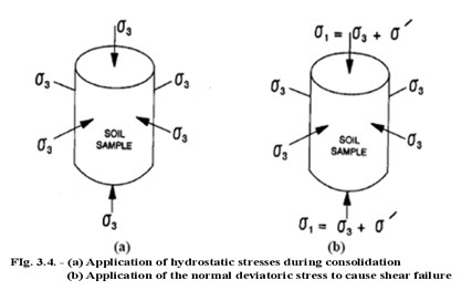
The deviator stress is increased until the soil fails. Figure 3.5(a) shows a two dimensional representation of stresses on the soil specimen. The soil failure plane orientation is shown by an angle (θ) from the horizontal. Figure 3.5(b) shows the shear and the normal stresses on the failure plane. Since the specimen failed the shear stress on this plane is equal to the shear strength. We now have to determine the values of the shear stress (τ) and the normal stress (σ) on this plane. These stresses can be determined by means of Mohr’s circles as shown in Figure 3.6. Point A on the circle represents the failure plane. It should be noted that the angle or orientation of the failure plane is doubled in the Mohr’s diagram. The coordinates of this point are the shear and the normal stresses on the failure plane. Using this diagram the following relationships can be written for these stresses:
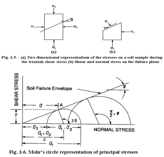
Figure 3.3 is a schematic diagram describing the triaxial apparatus and the application of stresses. The cylindrical soil specimen is enclosed within a thin rubber membrane and is placed inside a triaxial cell. The cell is then filled with a fluid. The specimen is subjected to a hydrostatic compressive stress (σ3) by pressurizing the cell. This causes the soil sample to consolidate. An additional vertical stress (σ') is applied through the piston as shown in the figure. This deviator stress is steadily increased until failure of the specimen occurs. The specimen fails under a set of principal stresses σ3 + σ' and σ3.
Drainage of water from the specimen is measured by a burette, and valve A can be closed to prevent drainage from the specimen. Another line from the base leads to a pressure sensor to measure pore water pressure.
To obtain the failure envelope, several triaxial tests are performed on specimens of the same soil at different values of cell pressure (σ3). A Mohr’s circle is drawn for the principal stresses at failure for each specimen. These are shown in Figure 2.10 and the line tangent to these circles constitutes the failure envelope. The stress on the failure surface is represented by the point of tangency. From the geometry of Mohr’s circle this plane makes an angle of (π/2 + ![]() )/2 with the major principal stress plane.
)/2 with the major principal stress plane.
The triaxial test may be performed as a drained (d), consolidated-undrained (c-u), or undrained test (u). In the drained test, water is allowed to seep out of the sample during the application of the hydrostatic and deviator stresses, and the pore water pressure is equal to zero. During the c-u test drainage is permitted during the application of the hydrostatic stress and the corresponding pore water pressure ua = 0. When the deviator stress is applied, drainage is not permitted and the pore water pressure ub > 0. In an undrained test, no drainage is permitted and the total pore water pressure is equal to u. The effective stress σ for the three drainage conditions may be calculated using the following equations:
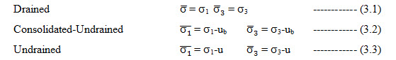
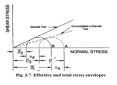
Figure 3.7 illustrates typical Mohr’s envelopes obtained from undrained, drained, and consolidated-undrained triaxial tests; the envelopes are constructed from the principal stresses at failure. The failure envelope corresponding to the drained test, called the effective failure envelope, may be determined from Equations 3.2 and 3.3 depending on the drainage condition of the test.
Regardless of the type of the test performed, there exists an effective failure envelope unique to the soil being tested. The effective-stress failure envelope is written as:
![]() ----------- (3.4)
----------- (3.4)
Shear strength of cohesionless soils.
Sand and silt are cohesionless soils. Figure 3.8 shows a typical failure envelope of a cohesionless soil.

The envelope passes through the origin. Thus, only one Mohr’s circle is needed to establish the failure envelope. The following equations are used to determine the drained (effective) failure envelope for cohesionless soils.
![]()
and ![]() ---------------- (3.6)
---------------- (3.6)
The value of ![]() for cohesionless soils ranges from about 28 to 42°. Generally, the value of
for cohesionless soils ranges from about 28 to 42°. Generally, the value of ![]() increases with increasing density. Extremely loose sands with an unstable structure may have a
increases with increasing density. Extremely loose sands with an unstable structure may have a ![]() as low as 10°.
as low as 10°.
Last modified: Wednesday, 12 February 2014, 9:39 AM