Mechanics of Tillage and Traction 3(2+1)

LESSON 12. PRINCIPLES OF SOIL CUTTING

12.2. Analysis of soil cutting and tillage

Basically, all soil cutting, moving and tillage instruments transfer soil from its original location. Thus the mechanical failure of the soil material is involved, in the sense that the mass of soil being moved does not retain its original geometric shape. The design of effective and efficient cutting tools begins with the analysis of this soil failure, in order to predict the forces and energy required by the implements. The design process proceeds subsequently to the description of soil manipulation and structural changes which result from cutting tool action, depending upon the special applications of interest.

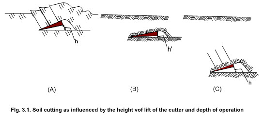
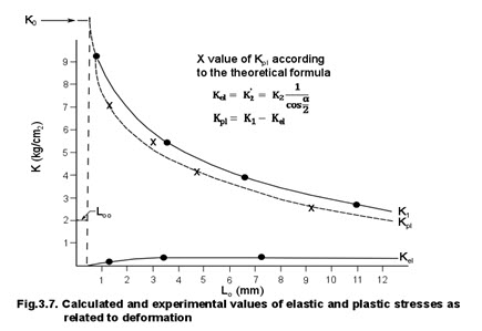
In situation A in figure 3.1, the lift height of the cutter is sufficient to cause shear failure surfaces that reach the surface of the soil. In situation B, however, the lift height of the cutter is not sufficient to displace the soil enough to cause major shear failure. In situation B, the soil mass separates with little evidence of any other action. Presumably, the soil was capable of absorbing the strain even though the same lift height as in situation A is used. To a certain degree, therefore, cutting as an action distinct from other failure of soil is determined by the degree of confinement in the neighborhood of the cutter. Obviously, the size of the required neighborhood for a specific cutter will be influenced by the condition of the soil. A wet plastic soil may cut in situation A of figure 3.1, whereas a dry brittle soil may create shear failure even with a low lift height as shown in situation B. Cutting as affected by degree of confinement was further demonstrated by Kostritsyn ( 230 ). He studied vertical rather than horizontal cutters. The cutters could be described as thin knives, and he observed the soil movement caused by the cutter. The results of his observations are shown in figure 3.1.

He noted that near the surface, soil would rupture or move upward (fig. 3.1-A); but at deeper depths, the movement was parallel to the direction of travel of the cutter. Figure 3.1, B shows the measured draft of the cutter versus the depth of the operation. Below a critical depth, a linear relation existed between draft and depth. The critical depth generally coincided closely with the observed depth where soil movement became horizontal. Kostritsyn reported that the critical depth was 20 to 25 centimeters for cutters approximately 3 centimeters thick. Thus, at deeper depths confinement of the soil causes pure cutting, whereas at shallower depths other types of soil failure also may occur. Kostritsyn described the soil movement near the surface as a crumbling action with the formation of crescent-shaped sliding bodies of soil. The description is similar to that used by Zelenin and Payne for vertical tools. Thus, although cutting can be clearly defined, in tillage tool operations it is not always clearly and independently involved. Obviously, a gradual transition from pure cutting to some complex action occurs as the depth of operation of a vertical cutter is decreased. A similar transition must occur when the depth of operation of a horizontal cutter is decreased or its lift height is increased at a constant depth of operation. Similarly, if soil conditions change from plastic to brittle, a transition from pure cutting to a complex action may occur. This lack of isolation of cutting has probably delayed its study, and no behavior equations have been developed to represent, cutting. As a consequence, no dynamic properties of soil associated with cutting have been identified.

Detailed studies of pure cutting have been made in the U.S.S.R., and Kostritsyn (230) continued the studies to a point where he developed a mechanics of cutting. His work followed the efforts of several earlier researchers, and he relied heavily on their findings. An interesting difference exists between the development of the mechanics of cutting and the development of the mechanics of inclined and vertical tools. In the latter mechanics, the reaction of the soil to a tool was visualized to result from simple behaviors that had been identified and were quantitatively defined. Thus, such factors as shear failure and soil-metal friction were used as the basis on which to establish a mechanics. Kostritsyn, on the other hand, directly analyzed the action and in the process developed a mechanics. He did not begin with behavior equations, but his mechanics implied the existence of a simple behavior equation. Kostritsyn’s success in developing his mechanics hinged on evaluating the implied behavior equation. While he recognized the behavior, he proceeded to evaluate it by indirect means rather than by a direct study of the behavior itself. Thus, he did not develop a simple behavior equation that, in turn, identified behavior properties of the soil. Kostritsyn did, however, manage to assess cutting of soil in empirical terms-that is, numbers that are some composite of the overall action involved in cutting rather than a clearly defined independent dynamic parameter. On this basis, he was able to construct his mechanics so that he could represent the action of cutting.

To illustrate the mechanics of cutting, Kostritsyn’s analysis is presented in detail. Kostritsyn restricted his attention to situations where only pure cutting was involved. In developing his mechanics he did not consider that any major failures other than separation were present. He considered two basic shapes of cutters (fig. 3.2).

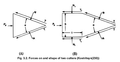
The leading angled edge of the cutters he designated as the wedge of the cutter while the parallel edges he called the sides. He reasoned that the forces acting on a cutter could be separated into several components and these components must be in equilibrium so that

P = P₁+P₂+P₃                                    ------------------ (3.1)

where  P = total force (draft) on the cutter,

P₁ = component of resistance resulting from the normal force on the wedge of the cutter,

P₂ = component of resistance resulting from the tangential force on the wedge of the cutter,

P₃ = component of resistance resulting from the tangential force on the side of the cutter.

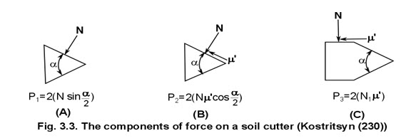
The forces are shown in figure 4, where N represents normal forces and T represents tangential forces. For a cutter shaped as shown in figure 3.2-A, obviously P3 in equation 3.1 will be zero. If the simple behavior of soil-metal friction is recognized, the tangential forces can be expressed in terms of the normal forces and friction is identified as the source of the tangential forces. Figure 3.3 shows the resistance forces resolved into horizontal components so that equation 3.1 can be written

              ------------- (3.2)

Where,

a = wedge angle of the cutter,

μ' = coefficient of sliding friction,

N = normal force on the wedge of cutter,

N₁ = normal force on the side of cutter.

With equation 3.2, Kostritsyn could calculate the cutting force for a particular cutter if he could specify the magnitude of the normal forces. By reasoning that these normal forces resulted from the resistance of the soil to deformation, he defined measures of the resistance so that

N = K₁F₁                                                                     ----------- (3.3)

Where,

K₁ = specific resistance to deformation,

F₁ = area of the wedge of cutter,

and

N₁ = K₂F₂                                                         ----------------- (3.4)

Where,

K₂ = specific pressure of soil,

F₂ = area of the side of cutter.

K2 differs from K1 in that K1 goes to zero when movement of the tool is stopped. K2, on the other hand, continues to press on the sides of the cutter even though the cutter is stopped ; it reflects an elastic type of restoration property in the soil. With equations 3.3 and 3.4, equation 3.2 can be rewritten to give

             ----------- (3.5)

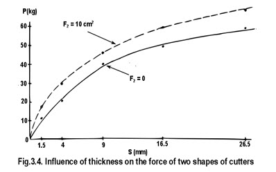
Equation 3.5 provides a means for experimentally studying cutting. For a specific cutter, the values of F₁, F₂, and μ' are known or can be determined and only K₁ and K₂ are unknown. By measuring P for a cutter shaped as shown in figure 4-A, K₁ can be evaluated from equation 3.5 since F₂ will be zero. If a similar cutter, but shaped as shown in figure 3.2-B is also used, the value determined for K₁ and equation 3.5 are sufficient to evaluate K₂. Figure 3.4 shows the difference in force on cutters of several thicknesses measured by Kostritsyn.

Having introduced the concepts of specific resistance and specific pressure (K1 and K2, respectively) that originate because the cutter causes the soil to deform, Kostritsyn took steps to evaluate the amount of soil deformation caused by a given cutter. He accepted as a working hypothesis the results of earlier Russian researchers who demonstrated that the path of movement of a particle of soil follows the direction of the resultant force ie., the path of motion and line of action of the resultant force will coincide.

 

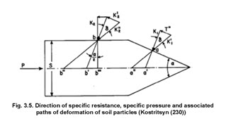
Figure 3.5 shows the paths of deformation for specific circumstances. If no friction occurs between the wedge of the cutter and the soil, a particle originally situated on the center axis of the direction of travel of the cutter will follow the path a'a shown in figure 3.5. During the forward movement of the cutter, the particle initially located at a’ will be moved along line a'a to a. Where soil metal friction is involved, the resultant force is inclined to the wedge by the angle of soil-metal friction In this case, a particle is moved along the line a''a, as shown in figure 3.5. The maximum displacement of soil thus is not equal to the width of the cutter S.Because of the interaction between the wedge angle and the soil-metal friction angle, the actual path length is something greater than S. Having established the direction of soil movement, Kostritsyn could calculate the maximum deformation for a given situation. The maximum occurs when point a in figure 100 reaches the widest part of the wedge section of the cutter. The maximum deformation is shown in figure 3.5 in the triangle bb''b’’’ where geometry indicates that the angle b''bb'' ' is (a/2 +d ) so that the length b''b is given by the equation

                         ----------- (3.6)

Where,

S = width of cutter,

d = angle of soil-metal friction,

a = wedge angle of cutter,

L_max   = maximum deformation.

The soil deformation along the wedge will vary from zero at the tip to the maximum shown in equation 3.6, so that average soil deformation L_o can be calculated by the relation

                                          ----------- (3.7)

Equation 3.7 applies to the deformation caused by the wedge portion of a cutter. Kostritsyn reasoned that no additional deformation occurs along the sides of the cutter, and the average deformation will be constant and numerically equal to that given for half of the maximum deformation occurring on one side of the cutter and expressed by equation 3.6.

Kostritsyn argued that a relation must exist between soil deformation, specific pressure, and specific resistance. In reality, specific pressure and specific resistance are the normal stresses acting between the soil and the cutter. The value of specific resistance is the stress required to cause a given deformation. Kostritsyn recognized that such behavior is stress-strain behavior (uniaxial compressive stress-longitudinal strain), but he also recognized that no suitable relation existed. Such a relation can be represented by a simple behavior equation that would define dynamic parameters of the soil. With the direction of strain movement specified as discussed (the behavior output of the equation) the mechanics of cutting could be developed in a manner similar to that used by Soehne, for example. Recognizing the behavior equations involved and specifying the behavior outputs establishes a method by which to locate and orient the forces involved.

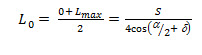
Kostritsyn, however, by analyzing the cutting reaction, has worked backwards and shown the need for a specific simple behavior equation. The difference that was discussed earlier between the methods for establishing a mechanics thus should be apparent. Kostritsyn did not study a stress-strain relation directly, but rather indirectly through his mechanics. For a given cutter he could calculate L_o for the respective K values from equations 3.6 and 3.7. He could evaluate experimentally the magnitude of the two K values from equation 85 by using two cutters with different shapes. An example of the relation between K₁ and K₂ and their respective average deformations is shown in figure 8 for one soil in one condition.

Several important conclusions by Kostritsyn are based on the general nature of the curves shown in figure 3.6. First, the two K values were not constant, so that they were not parameters assessing the soil. Since they represent stresses, constant values probably should not be expected. For the mechanics, however, a parameter must be found that is constant for a given soil condition. Second, the reversed trends for the two K values as the average deformation was increased indicate that some interaction between the soil and cutter must be occurring. If not, the trends should have been the same-they should both either increase or decrease as the average deformation increases.

 

Third, the low value of K₂ suggests that somehow the normal stress on the sides of the cutter is reduced during the soil reaction. To illustrate, we might reason that the maximum stress caused by the wedge of the cutter remains acting on the sides of the wedge as long as the soil is forced to remain deformed. In such circumstances, K₁ and K₂ should be related by the cosine of the angle of the wedge. As the data in figure 8 indicate, the implied angle of the wedge ranges from approximately 150° to 180º. Since these angles are completely unrealistic, a logical conclusion is that the stress on the sides of the cutter represented by K₂ is reduced by some type of relief. Based partly on the foregoing reasoning and partly on other observations, Kostritsyn proposed that the specific resistance and the specific pressure come from elastic and plastic deformations of the soil. He thus defined

K₁ = K_el+ K_pl                                                       ---------------- (3.8)

Where,

K_el = stress from elastic deformation,

K_pl = stress from plastic deformation.

He further considered that K₂ represented only the elastic deformation. These definitions imply that the soil deforms plastically and elastically as the wedge of the cutter advances. On the sides of the wedge, however, the soil has “adjusted itself” by plastic flow so that only the elastic rebound of the soil causes the stress. As figure 3.5 shows, the lines of action of the hypothesized stresses are not parallel but are related by the geometry of the cutter. Since the directions of K1 and K2 do not coincide, K₂ cannot be equated directly to the elastic component of stress in equation 3.8. From the geometry shown in figure 100, the magnitude of K2 in the K1 direction gives,

                         ----------------- (3.9)

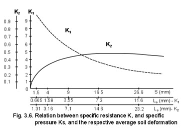
With equations 3.8 and 3.9, the elastic and plastic components of stress can be calculated from the values of K₁ and K₂. Figure 3.7 shows the respective values plotted against deformation, as determined by equation 3.7.  Kostritsyn determined the relation shown in figure 3.7 for several soils in various conditions.

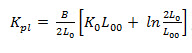
He concluded that the general shape of the curves was the same for all soils and then proceeded to obtain a mathematical expression for the curves. He noted that the relation between Kpl and Lo was very close to that of an equilateral hyperbola so he used the equation to express the relation.

  -------------------------------------- (3.10)

Close observation of the experimental data indicated that as L_o approached zero, the relation in equation 3.10 did not hold. This suggested that a minimum value for L_o existed and that it was equal to one or possibly several particle diameters. The minimum value L_oo represents a small distance that reflects the undeformable nature of individual soil particles.

Associated with this minimum deformation is the constant K_o given by

   ----------------------------------- (3.11)

Where,

L_oo = diameter of soil particles,

K_o = maximum stress to cause deformation.

Equation 3.10 was reasonably accurate as long as L_o was greater than L_oo. To overcome the restriction placed on equation 3.10, Kostritsyn used an equal area technique to evaluate the shape of curves and obtained the equation

                            ----------------------------(3.12)

Where,

B = coefficient of plasticity.

Kostritsyn then defined

K_el = K_o - K_pl   ------------------------------------- (3.13)   

and by using equation 16 and the equal area technique he obtained the equation

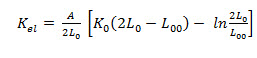             ---------------- (3.14)

where,

A = coefficient of elasticity.

Equations 3.12 and 3.14 take into account the restriction observed in equation 16. Coefficients A and B represent empirical constants that permit a more accurate representation of the relations between Kel, Kpl, and Lo. Note that in equations 3.12 and 3.14, A and B represent constants for a given soil condition, as do L_oo and K₀,. Thus, in a sense they are composite soil parameters. They are not, however, parameters of a behavior equation but rather of a mechanics for cutting.

Kostritsyn evaluated constants A and B for several conditions. For the soil represented in figure 3.7, he assumed Loo was approximately 0.5 millimeter. The coefficient B can be evaluated only from experimental data so that the value for K_pl at some arbitrary L_o is required. Given the value for B, K_pl can be determined for other values of L_o by using equation 3.12. The theoretical points shown in figure 3.7 were calculated from equation 3.12. Table 1 gives measured and calculated values for K_pl and K_el for a different soil condition. Kostritsyn stated that the large percentage of error at l-millimeter deformation was due to the inaccuracy of experimental apparatus for such small forces and deformations. As figure 3.7 and table 3.1 show, however, the experimental and calculated values agree remarkably well. Although Kostritsyn did not show data to compare the actual draft of the cutters, agreement of the soil stresses implies that the calculated and experimental drafts would have agreed just as well. Thus, the mechanics of cutting as developed by Kostritsyn is reasonably accurate and complete.

Table 3.1. Experimental and computed values of the plastic and elastic stresses to deformation during cutting

Mean soil deformation (mm)	Kpl			Kel
	Experimental values (Kg/cm2)	Computed values (Kg/cm2)	Difference (Kg/cm2)	Experimental values (Kg/cm2)	Computed values (Kg/cm2)	Difference (Kg/cm2)
1	7.3	5.60	- 2.5	0.212	0.330	+35
3	5.4	7.00	+3.5	0.390	0.405	+4
5	4.1	4.05	+1.0	0.440	0.440	0
10	2.5	2.50	0	0.465	0.465	0

SOURCE : Kostritsyn ( 230 ).

In order to determine parameters A and B, the forces on an actual cutter must, be measured experimentally. Therefore, the mechanics of cutting may seem to be a hoax. Such is not the case, however, if the means required to assess the magnitudes of A and B are recognized. As has already been implied, the parameters are defined by the mechanics rather than by a behavior equation. Kostritsyn argued that a stress-strain behavior equation must exist, but it is unknown. He proceeded to establish a relation indirectly through his mechanics where cutting is involved rather than a direct relation where the stress-strain behavior was isolated. His mechanics of cutting is thus the mathematical model that represents the situation under observation. The mathematical model defines parameters A and B; hence, they are parameters of the mechanics, not of stress- strain behavior.

The mechanics is the model and hence an actual cutter is required. Once A and B have been specified, however, they can be used and applied to that soil condition just as independent parameters such as cohesion can be applied. The mechanics of cutting thus differs from the earlier mechanics only in the method required to assess the respective soil parameters. While the mechanics seems to be very accurate as presented by Kostritsyn, caution should be used in its application. Stress-strain behavior is probably inaccurately represented because of the indirect manner in which it was studied. No distribution of stress is admitted to exist on the cutter when a distribution would seem logical. Whether the average stress and deformation accurately represent the implied behavior has not been determined.

Kostritsyn apparently confined his experiments to wet dense soils. Experience tells us that such soils tend to be plastic and therefore probably only pure cutting was involved in the experiments. In many soil conditions plastic behavior may be less evident and the relation expressed in equation 90 may be drastically different. If a difference occurs, equations 92 and 94 may no longer accurately represent the situation. Even further, this possibility raises the question as to whether pure cutting will be present. As soil conditions change so that plastic behavior is less dominant, other types of failure may also be present and increase in importance. Kostritsyn’s mechanics applies only to pure cutting and would not represent such situations. Considerations of this kind limit the situations where the mechanics can be applied.

A final consideration of the forces on a cutter suggest a possible component of resistance along the leading edge of the cutter. Such a force is present if large hard particles are visualized as being cut by an infinitely thin cutter, as shown in figure 3.8(A).

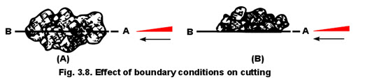
In order for the cutter to move from A to B along the projected path (fig. 3.8(A)), several of the large particles would have to be sliced and separated. Contrast this action to the actions mechanics for cutting, where particles presumably implied in Kostritsyn’s smaller than the cutter are merely displaced but not sliced. A possible fourth term could thus be included in equation 81. This term might be extremely useful when evaluating the cutting resistance of materials in the soil, such as roots. Figure 3.8 also shows the effect a boundary condition might have on cutting. If a pile of coal were being shoveled from the top (a situation similar to fig. 3.8(A)) rather than from a smooth floor (a situation similar to fig. 3.8 (B)), the force to push the shovel into the pile would obviously be different. In the latter case, the boundary condition becomes orderly so that cutting is not required. Shoveling from the top requires deforming the aggregate of coal in an action similar to that represented by Kostritsyn’s mechanics. The individual aggregates are displaced but not cut. Presumably an action could occur wherein the coal aggregates themselves would be severed so that an additional force would be required. Cutting per se is thus simply envisioned and easily defined, but its involvement with other actions compound and confuse the practical application of cutting. Getzlaff ( 142 ) has measured the effect of stones on the draft of plows and it appears that cutting or displacing rigid bodies can require considerable force.

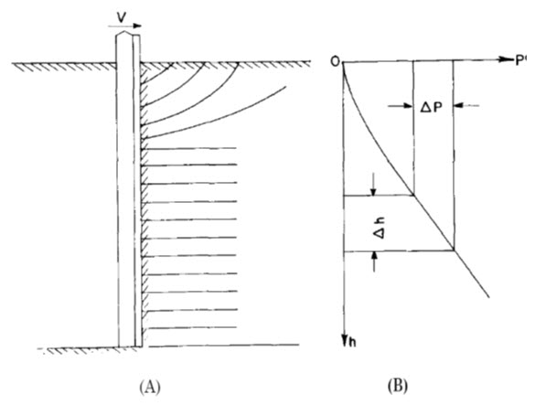
Fig 3.-A, Soil movement caused by a thin vertical cutter; B, relation of cutting force to depth of operation for a vertical cutter. (Kostritsyn ( 230 ).)