System Engineering 3(3+0)

LESSON 2. Investment Analysis

2. Break–Even Analysis

The break-even analysis is also known as cost-volume profit (CVP) analysis. The break-even analysis provides a relationship between revenues and costs with respect to volume (quantity) of sales or production. It represents the level of sales at which costs and revenues are in equilibrium; the equilibrium point being known as the break-even point (BEP). At the break-even point, total revenue is equal to the total costs, indicating  no-profit or no-loss point.

 2.1. Assumptions in break-even analysis

            The break-even analysis is based on the following assumptions: 

1. The total cost can be separated into fixed and variable costs.

2. The total fixed cost remains unchanged with changes in sales volume.

3. The variable cost per unit is constant and the total variable cost is proportional to the sales volume.

4. The selling price per unit is constant i.e., it does not change with volume.

5. The orgnaisation manufactures only one product or if there are multiple products, the sales mix does not change.

 Two following two methods are used to determine the break-even point: 

1. Formula method

2. The chart method

 2.2. Formula method

            The break-even point can be computed based on units, or in terms of money value of sales volume and  as percentage of estimated capacity.

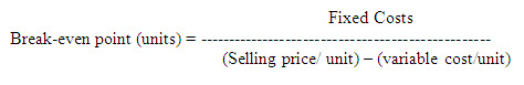
 2.2.1. Based on  unit

For an organisation with single-product, the break-even point in terms of units will be reached when the total earned revenue becomes equal to the total costs.

 Let,

s :   The unit selling price,

v :  The variable cost per unit,

F : The fixed costs, and

Q_B : The break-even point (units)

Then

Total revenue, R  = Q_B . s           .........(1)

Total costs, C     = F + Q_B . v     .......... (2)

             Therefore, at break-even point,

                        Q_B .s = F + Q_B .v                    .......... (3)

                         Or    

Q_B  =  F/(s-v)                          ............(4)

 Or                                                            

Fixed Costs

 2.2.2. In money value

The break-even point for a single-product organisation can also be expressesed based on  rupee value of sales volume. If both sides of equation (4) are multiplied by the unit selling price, s we get the break-even point, R_B  in terms of rupees. Thus

                   R_B = Q_B . s =  Fs / (s-v)          ................... (5)

or      

Break-even point (rupees) = R_B  =  F/ [1- (v/s)]                       (6)

As both the variable costs and sales revenue vary in direct proportion to sales volume, the above equation (6) can also be used for a multi-product organisation. For such organisatios, 

                                                                        Fixed costs

Break-even point (rupees) = --------------------------------------------------------

                                                1 – (Total variable costs / Total sales revenue)

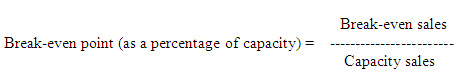
 2.2.3. Based on percentage of capacity

 The break-even point as a percentage of capacity is obtained by dividing the break-even sales by the total estimated sales or capacity sales. Thus

2.3. The chart approach

The break-even chart (Fig.1) represents a pictorial view of the relationships among costs, volume and profit. In this chart the break-even point is the point  at which the total cost line and the total sales line intersect. The break-even chart is constructed as given below.

1. Represent the sales revenue along the horizontal axis. The sales revenue may be expressed in terms of units, rupees or as a percentage of capacity. 

2. Represent the revenue, fixed and variable costs along the vertical axis. A similar vertical line may be drawn on the right of the chart to complete the square. 

3. Draw the fixed cost line parallel to the horizontal axis through the fixed cost point. 

4. Draw the total sales line and the total cost line. The point at which they intersect is the break-even point. The angle between these lines is called the angle of incidence. Larger this angle, lower the break-even point and vice-versa. The area to the left of this point is the loss area and represents the unrecovered fixed costs, while the area to its right is the profit area.

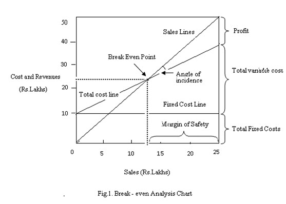
The excess of actual or budgeted sales over the break-even sales is called margin of safety. The margin of safety ratio is expressed as,

               Margin of safety  ratio=   (Budgeted sales – Break even  sales) / Budgeted sales

 The margin of safety indicates the extent to which sales may fall before a firm suffers a loss. Larger the margin of safety, safer the firm.

 2.4. Utility of break-even analysis

 Break-even analysis is the most useful technique of profit planning and control. It is a device to explain the relationship between cost, volume and profits. The utility of the break-even analysis lies in the following advantages it has: 

1. It is a simple device to understand complicated accounting data. 

2. It is a simple diagnostic tool. It indicates the management,  the causes of increasing break-even point and falling profits  to take appropriate actionn. 

3. It provides basic information for further profit improvement studies and is a useful starting point for detailed investigations. 

4. It is an useful method for considering the risk implications of alternative actions. From while another alternative may produce comparatively. Lower profit but may also entail a lower break-even point. In taking a decision, the firm should not only consider the profits expected from the alternative but also the probability of reaching the break-even point is higher should be preferred.

2.5. Limitations of break-even analysis 

1. It may be difficult to separate costs into fixed and variable components.

2. The total fixed cost may not remain unchanged over the entire volume range.

3. The unit selling price and unit variable cost may not remain constant.

4. It is difficult to use for a multi-product firm.

5. It is a short-term concept and has limited use in long-term planning.

6. It is a static tool and shows the relationship among costs, volume and profits of an organisation at a given point of time only.

3. Payback Period Method

 Payback period is the most popular method of evaluating investment proposals. It is defined as the number of years required to recover the cash invested in a project. If the annual cash inflows are same, the payback period is computed by dividing cash invested by the annual cash inflow; if unequal, it is calculated by adding up the cash inflows until the total is equal to the initial cash invested.

If the payback period calculated for a project is less than the maximum payback period set  by the management, the project is accepted; if not, it is rejected. By  ranking method it gives the highest ranking to the project that has the shortest payback period and lowest ranking to the project with the highest payback period.

 The merits of this method are:

1. It is simple to understand and easy to calculate.

2. It is less costly than the other evaluation techniques. Demerits:

3. The cash inflows that accrue after the payback period is not accounted.

4. It fails to consider the magnitude and timing.

4. Average (Accounting) Rate of Return Method

The accounting rate of return (ARR) is found by dividing the average annual net income (after taxes and depreciation) by the average cash outlay i.e., average book value after depreciation. The accounting rate of return is thus an average rate and can be determined by the following equation:

 Average income

ARR    =  ----------------------------------

                     Average investment

             A variation of ARR method is to divide the average earnings after taxes by the original cost of the project instead of average cost.

This method accepts all those projects whose ARR value is higher than the minimum rate established by the management and rejects those whose ARR value is lower. It also ranks the project as number one if it has highest ARR and lowest rank would be assigned to the project with lowest ARR.

 The merits of this method are: 

1. It is very simple to understand and use.

2. It can be easily calculated using the accounting data.

3. It uses the entire stream of incomes in calculating the accounting rate

 The demerits of this method are: 

1. It uses accounting profits and not cash flows in comparing the projects.

2. It ignores the time value of money. Profits accruing in different periods are valued equally.

3. It does not allow for the fact the profits can be reinvested.

5. Time – Adjusted 0r Discounted Cash Flow (DCF) Methods

 The above methods discussed suffer from drawback that they fail to recognize the time value of money in evaluating the investment worth of the projects.

Methods that fully recognise the time value of money are called time-adjusted or discounted cash flow or present value methods. They are 

1. Net present value method
2. Internal rate of return method 

5.1. Net present value (NPV) method 

This method fully recognises the time value of money. It correctly postulates that cash flows arising at different time periods differ in values and are comparable only when their equivalents-present values-are found out. It involves the following steps. 

1. Select an appropriate rate of interest to discount cash flows. Generally this rate is the firm’s cost of capital which equals the minimum rate of return expected by the investor.

2. Compute present value of cash inflows and outflows using the cost of capital as the discount rate. If all cash outflows are made in the initial year, then their present value will be equal to the cash actually spent.

3. Find out the present value by subtracting the present value of cash outflows from the present value of cash inflows.

4. Accept the investment project if its net present value is positive or zero and reject it if its net present value is negative. 

The equation for NPV, assuming that all cash outflows are made in the initial year t_o can be written as

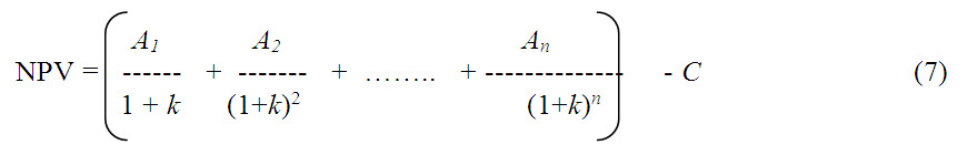
                    _n         A_t

              =  Σ   ------------ - C                                                                                        (8)

                 ^{t =1}      (1 + k)¹

 where A₁, A₂, ........ A_n  represent the cash inflows, k is the firm’s cost of capital, C is the outlay and n is the expected life of the proposal.

 The merits of this method are:  

1. It recognises the time value of money.

2. It considers all cash flows over the entire life of the project.

3. It aims at maximizing the welfare of the owners of the organization.

The demerits of this method are: 

1. It is difficult to use.

2. It assumes that the discount rate – which is usually the firm’s cost of capital – is known; but the cost of capital is difficult to understand and measure.

3. It may not give satisfactory answer when projects involving different amount of investment are compared. The project with higher NPV may not be desirable if it also requires a large investment.

 5.2. Internal rate of return (IRR) method

The internal rate of return is the rate that equals the present value of cash inflows with the present value of cash outflows of an investment. Thus it is the rate at which the net present value of the investment is zero. It can be determined from the following equation:

 

                        A₁                   A₂                                            A_{n                 n}       A_t

            C =  ----------- +  ----------  + …….+   ------------   =  Σ  ---------                       (9)

                      1 +  r            (1+r)²                       (1+r)^{n              t =1}  (1 + r)^t

  _n        A_t

or         Σ  ---------  -  C  =  0                                                                                        (10)

                  ^{t =1}  (1 + r)^t

It may be seen that the IRR formula is the same as used for the NPV method with the difference that in the NPV method the required rate of interest (cost of capital), k is known and the NPV is to be found out, while in the IRR method the value of r is to be determined at which the NPV is zero. The value of r in the IRR method the value of r is to be determined by trial and error method. Some value of the rate of return is chosen and NPV of cash inflows is calculated. If this value is lower than the present value of cash outflows, a lower rate is tried; if this value is higher than the present value of cash outflows, a higher rate is tried. The process is repeated until the net present value becomes zero. 

According to IRR method, a project is accepted if its internal rate of return is higher than or equal to the minimum required rate of return (i.e., r ≥ k); and the project is to be rejected if r < k.

 Merits: 

1. Like the NPV method, it considers the time value of money.

2. It considers cash flows over the entire life of the project.

3. It has psychological appeal to the users.

Demerits: 

1. It is difficult to understand and use in practice.

2. It may yield results inconsistent with the NPV method if the projects differ in their expected lives or cash outlays or timing of cash flows.

3. It may not give unique answers in all situations.

6. Discounted Payback Period Method

 The payback period is defined as the number of years required to recover the original cash investment in a project. In case of the discounted payback period, we consider the discounted present values of future cash inflows and determine the number of years required to recover the initial investment. If discounted payback period is less than the desired payback period, the project is accepted, otherwise it is rejected.

 7. Investment Decisions

 Investment decisions are taken on the time value of money and principles of equivalence. The money inflows and outflows at various points should not be added as such but should be reduced to a common point and added. For performing certain operations may be many methods available and are considered as equivalent methods. Among these methods, it is decided to choose based on the time value of money. It may be an equipment/ machinery for doing the given job. When number of such equipment or machinery are available the suitable one is selected based on the analysis of time value of money.   The following steps are involved in making the investment decision.  

i.  identification of alternative

ii. get the cash flow

iii. taking the decision based on the time value of money following any of the following methods 

a. equivqlent annual cost

b. present worth

c. internal rate of return

 Let P be the present worth of an investment and over a period of n it yields to F, further worth, if it is the compound interest. For the given P or F, the equivalent considerable worth is A. These terms, A, F and P are connected through the following relations for taking investment decisions. 

 If P is the sum at time 0 and F is the value after n years, 

 the value of P at end of 1^st year,        F₁ = P+P_i  = P(1+i)

                                      2^nd year,        F₂ = P(1+i) (1+i) = P(1+i)²

                                      n^th year ,       Fn = P(1+i)ⁿ  =  F

                                                     

F = P (1+i)ⁿ                                                    (11)

P = F (1/1+i)ⁿ                                                 (12)

(1+i)ⁿ is called single payment compound amount factor, (F/P, i, n)

(1/1+i)ⁿ  is called single payment present worth factor (P/F, i, n)

 If A  is the amount paid every year for a period of n years @ i, at the end of n years, the value will be,

              F = A [1+(1+i) +(1+i)² + ………….+ (1+i)^n-1]                              (13)

 where the amount paid during 0,1,2,…periods will earn interest for  n, n-1, n-2,… years.

 Multiplying both the sides by,  (1+i)

 F(1+i)  = A [(1+i) +(1+i)² + (1+i)³ ………….+ (1+i)ⁿ]                            (14)

 (14) – (13),

   -F + iF + F = A [-1 + (1+i)ⁿ]

           

                  F = A [(1+i)ⁿ-1/i]                                                                    (15)

 

                  A = F [i/(1+i)ⁿ-1]                                                                    (16)

[(1+i)ⁿ-1/i] is called uniform series compound amount factor (F/A).

[i/(1+i)ⁿ-1] is called sinking fund factor (A/F).

 substituting  (1) in (16),

 A = P(1+i)ⁿ [i/(1+i)ⁿ-1]   

                  A = P [i(1+i)ⁿ / (1+i)ⁿ-1]                                                         (17) 

                  P = [(1+i)ⁿ-1/ i(1+i)ⁿ]                                                             (18)     

 

[i(1+i)ⁿ / (1+i)ⁿ-1] is called  capital recovery factor (A/P).

[(1+i)ⁿ-1/ i(1+i)ⁿ] is called uniform series present worth factor (P/A).

A packaging operation in a food industry was performed using manual labour which involves Rs.50,000 per year as wages. The same can be performed by employing a packaging machine which costs Rs.1,00,000/- and requires one labour only. The expenditure towards electricity and spares repaired and labour charges are Rs.5000, Rs.10,000 and Rs.10,000 respectively. Suggest the industry whether to go for packaging machine. The life of the machine is 10 years and the scrap value is 10% of interest  rate is 12%.

 Equivalent Annual Cost Method

 

Plan A (Manual method): 

Annual expenditure on labour,  A_L   = Rs. 50,000

Equivalent annual cost,               A_A  = Rs. 50,000

 

Plan B (Using the packaging machine) 

Investment for packaging machine at 0 time, P = Rs. 1,00,000

Annual labour cost,                             A1 = Rs. 10000

Annual cost for electricity,                 A2 = Rs. 5000

Annual cost for spares and repair,      A3 = Rs. 10000

Annual cost of total expenditure,          A = Rs. 25,000

 

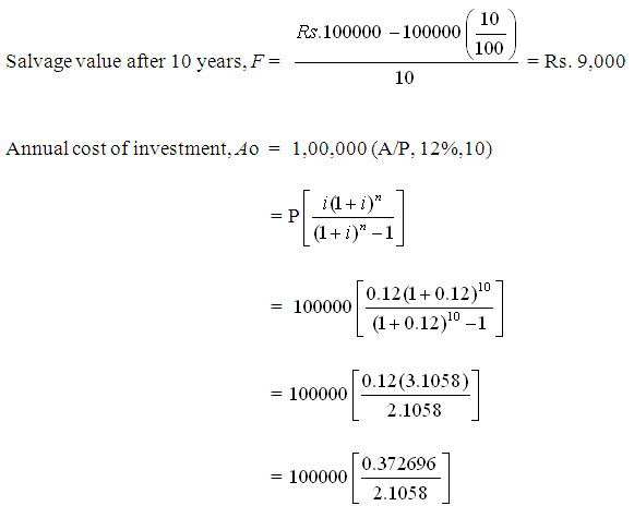
                                                               = 100000[0.177]    = Rs. 17700

Annual cost of scrap value, A_S  =  9000 (A/F, 12%, 10)

                                                  

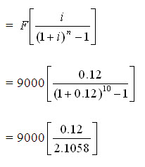
                                                   = 9000 [0.05698]  = Rs. 513 

Total equivalent annual cost of the investment,  A_B = A + A_O +A_S 

                                                                            = 25000 +  17700  + 513 

                                                                             = Rs. 43,213 

Since the equivalent annual cost of plan B is less, plan B is suggested.

Present worth method

Plan A

Annual expenditure on labour,           A = Rs. 50,000

Present worth of the annual cost,       P = Rs. 50,000 (P/A, 12%, 10)

                                                        

                                                           = 50000 [5.6502]                                                          

                                                           = Rs.2,82,510 

Plan B

Present worth of the investment at 0 time,     P₁ = Rs.1,00,000

Equivalent annual cost of expenditure,          A = Rs.25,000

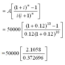
Present worth of annual expenditure,                         P₂ = 25,000 (P/A, 12%, 10)

 

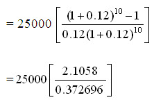
                                                                 = 25000 [5.6502]                                                          

                                                                 = Rs.1,41,255

Scrap value at the end of 10 year, F = Rs.9,000

Present worth of scrap value, P₃ = 9,000 (P/F, 12%, 10)

 

                                                   = 9000[0.322]              

                                                   = Rs. 2,898

Total present worth of plan B, P = P₁ + P₂ +P₃ 

                                                    =  1,00,000 + 1,41,255 + 2,898 

                                                    = Rs.2,44,153

 Since the present worth of plan B is less, plan B  is suggested.