System Engineering 3(3+0)

LESSON 1. Assignment problems - Introduction

1. Introduction

The assignment problem is defined as  assigning each facility to one and only one job so as to optimize the given measures of effectiveness, when n facilities and n jobs are available and given the effectiveness of each facility for each job.

Let there be  n facilities (machines) to be assigned to n jobs. Let c_ij is cost of assigning i^th facility to j^th job and x_ij  represents the assignment of i^th facility to j^th job. If i^th facility can be assigned to j^th job, x_ij=1, otherwise zero. The objective is to make assignments that minimize the total assignment cost or maximize the total associated gain.

  

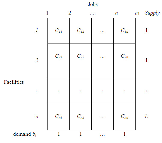
Thus an assignment problem can be represented by n x n matrix which continues n! possible ways of making assignments. One obvious way to find the optimal solution is to write all the n! possible arrangements, evaluate the cost of each and select the one involving the minimum cost. 

However, this enumeration method is extremely slow and time consuming even for small values of n. For example, for n = 10, a common situation, the number of possible arrangements is 10! = 3,628,800. Evaluation of so large a number of arrangements will take a probability large time. This confirms the need for an efficient computational technique for solving such problems.

 2. Mathematical Representation of Assignment Model

 Mathematically, the assignment model can be expressed as follows: 

Let x_ij  denote the assignment of facility i to job j such that

                        x_ij = 0, if the i^th facility is not assigned to j^th job,

                        x_ij = l, if the i^th facility is assigned to j^th job.

Then, the model is given by

             

            subject to constraints   

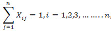(one job is assigned to the i^th facility)         

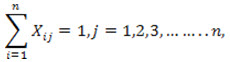                          (one job is assigned to the j^th facility)                                                      

 

and                  x_ij  = 0  or 1 (or x_ij = x_ij²).

 If the last condition is replaced by x_ij ≥0, this will be a transportation model with all requirements and available resources equal to 1.

3. Comparison with the transportation model

An assignment model may be regarded as a special case of the transportation model. Here, facilities represent the ‘sources’ and jobs represent the ‘destinations’. Number of sources is equal to the number of destinations, supply at each source is unity (a_i = 1 for all i) and demand at each destination is also unity (b_j = 1, for all j). The cost of ‘transporting’ (assigning) facility i to job j is c_ij and the number of units allocated to a cell can be either one or zero. i.e., they are non-negative quantities.

However the transportation algorithm is not very useful to solve this model, when an assignment is made, the row as well as column requirements are satisfied simultaneously (rim conditions being always unity) resulting in degeneracy. Thus the assignment problem is a completely degenerate form of the transportation problem. In n x n problem, there will be n assignments instead of n+n–1 or 2n–1–n = n–1 epsilons which will make the computations quite cumbersome. However, the special structure of the assignment model allows a more convenient and simple method of solution.

 

Difference between the transportation problem and the assignment problem

	Transportation Problem	Assignment Problem
(a)	Supply at any source may be any positive quantity ai	Supply at any source (machine) will be 1 i.e., ai =1.
(b)	Demand at any destination may be any positive quantity bj	Demand at any destination (job) will be 1 i.e., bj = 1.
( c)	One or more source to any number of destinations	One source (machine) to only one destination (job).

 

4. Theorems

The technique used for solving assignment model makes use of the following two theorems:

4.1. Theorem I

It states that in an assignment problem, if we add or subtract a constant to every element of a row (or column) in the cost matrix, then an assignment which minimizes the total cost on one matrix also minimizes the total cost on the other matrix”.

Let, c_ij represent the original cost elements of the matrix. If constants u_i and v_j are subtracted from the i^th row j^th column respectively, the new cost elements will be

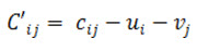
If Z is the original objective function, the new objective function will be

                          

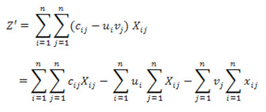
  Now with reference,                            

                       

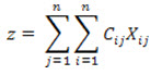
 and

                   

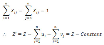
         or z' is minimum when z is minimum. This proves the theorem.

 Likewise, if in an assignment problem some cost elements are negative, we may convent them into an equivalent assignment problem where all the cost elements are non-negative by adding a suitably large constant to the elements of the relevant row.

 4.2. Theorem II

 It states “If all c_ij ≥ 0 and we can find a set x_ij=x’_ij,  such that

     

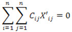
 then this solution is optimal.

 The result follows automatically since as neither of c_ij is negative, the value of

                           cannot be negative.

Hence, its minimum value is zero which is attained when x_ij=x_ij' . 

Thus the present solution is optimal solution.

The above two theorems indicate that if one can create a new c_ij' matrix with zero entries, and if these zero elements, or a subset thereof, constitute feasible solution, then this feasible solution is the optimal solution.

 Thus the method of solution consists of adding and subtracting constant from rows and columns until sufficient number of c_ij's become zero to yield a solution with a value of zero.