System Engineering 3(3+0)

LESSON 2. Assignment problems - Solutions of the assignment problems

                    

 

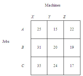
If job A is assigned to machine X,  the cost of this assignment is Rs. 25. Since machine Y can also process job A for Rs. 15, clearly assigning job A to machine X is not the best decision. Therefore, when job A is arbitrarily assigned to machine X, it is done by sacrificing the opportunity to save Rs. 10 (Rs. 25 – Rs. 15). This  sacrifice is referred to as an opportunity cost. The decision to process job A on machine X precludes the assignment of this job to machine Y, given the constraint that one and only one job can be assigned to a machine. Thus opportunity cost of assigning job A to machine X is Rs.10 with respect to the lowest cost assignment for job A. Likewise, a decision to assign job A to machine Z would involve an opportunity cost of Rs. 7 (Rs. 22 – Rs. 15). Theassignment of job A to machine Y is the best assignment as the opportunity cost of this assignment is zer (Rs.15-Rs.15). This is called the  machine – opportunity costs with regard to job A. Similarly, if the lowest cost of row B is subtracted from all the costs in this row,   the machine-opportunity costs for job B can be obtained. By following the same step, the machine opportunity cost for job C can be obtained . This is given in the following table.

                             

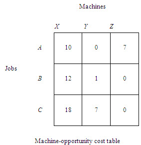
In addition to these machine-opportunity costs, there are job-opportunity costs also. Job A, B and C, for instance, could be assigned to machine X. The assignment of job B to machine X involves a cost of Rs. 31, while the assignment of job A to machine X costs only Rs. 25. Therefore, the opportunity costs of assigning job B to machine X is Rs. 6 (Rs. 31 – Rs. 25). Similarly, the       opportunity cost is involved in the assignment of job A to machine X is Rs. 10 (Rs. 35 – Rs. 25). A zero opportunity cost is involved in the assignment of job A to machine X, since this is the best assignment for machine X (column X). Hence job-opportunity costs for each column (each machine) are obtained by subtracting the lowest cost entry in each column from all cost entries in that column, if the lowest  entry in each column  of table is subtracted from all the cost entries of that column, the resulting table is called total opportunity cost table.

           

                               Machines

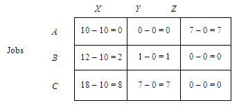
                          Total opportunity cost table

The objective is to assign the jobs to the machines to manimize total costs. With the total opportunity cost table this objective will be achieved if the jobs are assigned to the machines in such a way as to obtain a total opportunity cost of zero. Four cells in the total opportunity cost table contains  zeros, indicating a zero opportunity cost for these  cells (assignment). Hence job A could be assigned to machine X or Y and job B to machine Z, all assignments having zero opportunity costs. This way job C, however, could not be assigned to any machine with a zero opportunity cost since assignment of job B to machine Z precludes the assignment of job C to this machine. Clearly, to make an optimal assignment of the three jobs to the three machines, there must be three zero cells in the table such that a complete assignment to these cells can be made with a total opportunity cost of zero. 

Drawing minimum number of lines covering all zero cells in the total opportunity cost table with minimum number of lines equals the number of rows (or columns) in the table is  a convenient method for determining whether an optimal assignment is  made  If, however, the minimum number of lines is less than the number of rows (or columns), an optimal assignment cannot be made. In this case there is  need to develop a new total opportunity cost table. In the present example, since it requires only two lines to cross (cover) all zeros, and there are three rows, an optimal assignment is not possible. Clearly, there is a need to modify the total opportunity cost table by including some assignment not in the rows and columns covered by the lines. Of course, the assignment chosen should have the least opportunity cost. In the present case it is the assignment of job B to machine Y with an opportunity cost of 1. In other words, we would like to change the opportunity cost for this assignment from 1 to zero.

           

             Machines

            

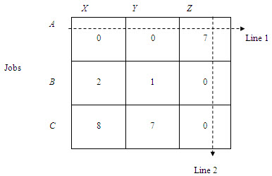
To accomplish this (a) choose the smallest elements in the table not covered by a straight line and subtract this element from all other elements not having a line through them (b) add this smallest element to all elements lying at the intersection of any two lines. The revised total opportunity cost table is shown below.

 

 Machines

   

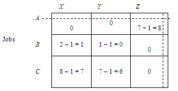
Revised opportunity cost table

 

The test for optimal assignment described above is applied again to the revised opportunity cost table. As the minimum number of lines covering all zeros is three and there are three rows (or columns), an optimal assignment can be made. The optimal assignments are A to X, B to Y and C to Z.

In larger problems there is need for more systematic procedure, as the assignments may not be readily apparent.