Strength of Material 3(2+1)

LESSON 3. Deflection of Beam: Direct Integration Technique - 1

3.2 Differential Equation for the Elastic Line

Consider a beam (Figure 3.1a) undergoes transverse deformation as shown in Figure 3.1b. As a result of this deformation fibers on the convex side of the beam are elongated while those on the concave side are shortened. Somewhere in between top and bottom of the beam, there is a layer of fibers which remain unchanged in length. This neutral layer is called neutral surface and intersection of the neutral surface with the axial plane of symmetry is called neutral axis.

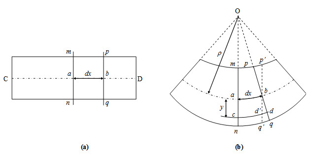
Fig. 3.1.

The deformed configuration of the neutral axis is called the elastic line or deflection curve. In this section we will derive the differential equation of this elastic line. The assumptions which constitute the basis of the derivation are given bellow.

• Material is homogeneous and obeys Hooke’s law.
• The curvature is small.
• Any cross-section originally plane and normal to the neutral axis is assumed to remain plane and normal to the neutral axis during the deformation.

Consider an infinitesimal segment dx between two adjacent cross-section mn and pq in undeformed configuration as shown in Figure 3.1b. After deformation, mn and pq no longer remain parallel and let they intersect at O at an angle dq as shown in Figure 3.1b. Now the relation between dx and dq may be written as,

\[d\theta=dx{1 \over \rho }\]                                                (3.1)

where \[{1 /\rho }\]  is the curvature of the neutral axis of the beam.

Now consider a fiber cd at a distance y from the neutral axis and having initial length dx. After deformation it elongates by amount. Therefore longitudinal strain in fiber cd may be expressed as,

\[{\varepsilon _x}={{dd'} \over {dx}}={{yd\theta } \over {dx}}={y \over \rho }\]                                                            (3.2)

It is to be noted that if a fiber on the concave side of the neutral axis is considered, the distance y will be negative and consequently the strain is also negative. Now position and curvature of the neutral axis may be determined by using equilibrium condition as follows.

3.2.1 Position of the Neutral Axis

Following the Hooke’s law the longitudinal stress (bending stress) may be written as,

\[{\sigma _x}=E{\varepsilon _x}={E \over \rho }y\]                                                       (3.3)

where E is the Young’s modulus. Equation (3.3) shows that the fiber stress varies linearly across the depth of the beam with maximum and minimum values at the two extreme (bottom and top) fibers and zero at neutral axis as shown in Figure 3.2.

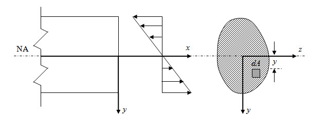
Fig. 3.2.

Now force on an infinitesimal area dA at a distance y from the neutral axis is. Since there is no normal force in the longitudinal direction, force equilibrium condition in the longitudinal direction may be written as,

\[\int\limits_A {{\sigma _x}dA}=0 \Rightarrow {E \over \rho }\int\limits_A {ydA}=0 \Rightarrow \int\limits_A {ydA}=0\]                         (3.4)

In the above equation,  \[\int\limits_A {ydA}\]  is the moment of area about z-axis (see Figure 3.2) which may also be expressed as \[A{y_c}\]  where \[{y_c}\] is the distance of centroid from the neutral axis. Since \[A \ne 0\]  , from equation (3.4) we have  \[{y_c}=0\]  . Therefore neutral axis of the cross-section passes through its centroid.

3.2.2 Curvature of Neutral Axis

Curvature of the neutral axis may be determined from the condition that the resulting couple induced by the longitudinal stress  must be equal to the bending moment M. Therefore,

\[M=\int\limits_A {y{\sigma _x}dA}\Rightarrow M={E \over \rho }\int\limits_A {{y^2}dA}\Rightarrow {1 \over \rho }={M \over {EI}}\]        (3.5)

where \[I=\int\limits_A {{y^2}dA}\] is the second moment of area of the cross-section about z-axis.

If we consider the deflection curve as a smooth function of x, its curvature may be written as,

\[\frac{1}{\rho } = \frac{{\left| {\frac{{{d^2}y}}{{d{x^2}}}} \right|}}{{{{\left[ {1 + {{\left( {\frac{{dy}}{{dx}}} \right)}^2}} \right]}^{3/2}}}}\]  (3.6)

For small deflection, slope \[{{dy}{\left/ {dx}}\]   is very small as compared to unity and hence the curvature may be approximated as,

\[{1 \over \rho }=\left| {{{{d^2}y} \over {d{x^2}}}} \right|\]                                               (3.7)

Combining equation (3.5) and (3.7), we have,

\[\left| {{{{d^2}y} \over {d{x^2}}}} \right|={M \over {EI}}\]                                              (3.8)

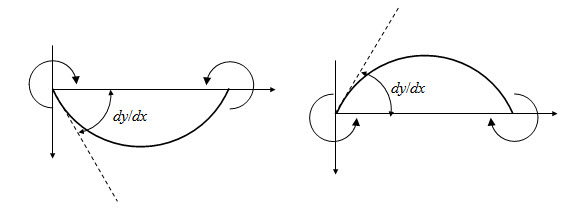Fig. 3.3. (a) Moment positive, curvature concave upward; Moment negetive, curvature concave downward.

As illustrated in Figure 3.3, when moment is positive, slope  \[{{dy}/ {dx}}\]  algebraically decreases ( \[{{{d^2}y}/ {d{x^2}}}\]  is negative) with x and vice versa. Therefore equation (3.8) may be recast as,

 \[{{{d^2}y} \over {d{x^2}}}=- {M \over {EI}}\]                                                             (3.9)

Equation (3.9) is the differential equation of the elastic line for a beam. Following forms of equation (3.9) are also found useful especially when load has non-uniform distribution.

\[{d \over {dx}}\left( {EI{{{d^2}y} \over {d{x^2}}}} \right)=- {{dM} \over {dx}} \Rightarrow {d \over {dx}}\left( {EI{{{d^2}y} \over {d{x^2}}}} \right)=- V\]          (3.10)

\[{{{d^2}} \over {d{x^2}}}\left( {EI{{{d^2}y} \over {d{x^2}}}} \right)=- {{dV} \over {dx}} \Rightarrow {{{d^2}} \over {d{x^2}}}\left( {EI{{{d^2}y} \over {d{x^2}}}} \right)=q\]               (3.11)

where V is the shear force and q is the intensity of the distributed load at any cross-section. Deflection of beam may be determined by solving any of equation (3.9) – (3.11). This will be discussed in next lesson.

 

Suggested Readings

Hbbeler, R. C. (2002). Structural Analysis, Pearson Education (Singapore) Pte. Ltd.,Delhi.

Jain, A.K., Punmia, B.C., Jain, A.K., (2004). Theory of Structures. Twelfth Edition, Laxmi Publications. 

Menon, D.,  (2008), Structural Analysis, Narosa Publishing House Pvt. Ltd., New Delhi.

Hsieh, Y.Y., (1987), Elementry Theory of Structures , Third Ddition, Prentrice Hall.