Farm Power & Machinery Management 3(2+1)

Lesson 15 and 16. Selection of tractors

A successful farm machinery system is one that must perform in such a manner that profit to the farm is maximized. Maximization is not always accomplished by minimizing costs, and such is true with the selection of a farm machinery system. Considerations have to be given to the economic value of operating machinery at that correct moment of time when the soil, the crop, the weeds, and the insects are most affected. The need for timely operations is a rather unique economic constraint on the farm machinery system.

Selection of an appropriate machinery system may be stated simply as the process of determining those individual machine capacities, which will optimize the economic performance of the whole system. Consideration must be given to machine costs, power costs, operational costs etc.  An appropriate cost of operation model is essential to the validity of the selection problem analysis. This analysis uses fixed and variable costs.  Variable costs increase proportionally with the operational use of the machine, while fixed costs are independent of use.  Considering the fixed and variable costs, the total cost of operation of tractor is given by

Ac       =          Fc Pt  +  At ( RM + L + O + F + Tc )      ------------  (1)

Where,

Ac       =          Annual costs of operating the tractor, Rs/year

Fc        =          Annual fixed costs, fraction of purchase price

Pt         =          Purchase price of tractor, Rs

At        =          Annual use of tractor, h/year

RM      =          Repair and maintenance costs of tractor, Rs/h

L          =          Labour costs, Rs/h

O         =          Oil costs, Rs/h

F          =          Fuel costs, Rs/h

Tc        =          Timeliness costs, Rs/h

Since RM , O , F = f(A) where A is cropped area, therefore, RM , O , F = f(E) where E is energy spent to cover the area . As energy requirement is expected to be a constant for a specific farm operation, therefore, RM, O and F costs will have no influence on the optimum size of the tractor. Thus, only important variables are labour costs (L) and timeliness costs (Tc). More specifically, the annual costs of tractor are expressed as the sum of the fixed costs and the total labour and timeliness costs for each of two types farm jobs viz. field operations and transport operations.

Ac  =   Fc Pt  +  (Field hours) (L+ timeliness cost) + (transport hours) (Lt)

Where,

L          = Tractor operator’s wages for field work, Rs/h

Lt        = Labour cost for transport work, Rs/h

Probably, there should be a timeliness charge for transport work but for simplicity it will be assumed that this does not limit field operation.

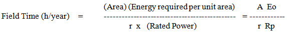
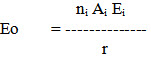
The optimum size of tractor is considered to be one, which will perform all the desired operations at minimum costs.  The annual hours of work required for each class of tractor operation are given by:

Where,

A         = Area, ha

r           = Ratio of drawbar power to rated engine power for drawbar loads  and ratio of PTO power to rated engine power for PTO  loads

Eo        = Energy required per unit area, kWh/ha

Rp       = Rated power, kW

Thus field time is proportional to energy required per unit area per rated power i.e.

Field Time =  C₁ Eo/Rp

Where,

C₁        =          Constant

Similarly;

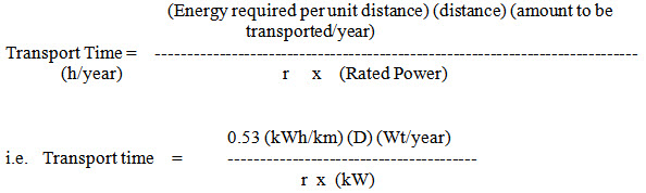
Where,

Wt       =          Amount of material to be transported, tonne

D        =          Distance to be travelled, km

r          =          Ratio of drawbar power to rated engine power taken as 0.4 for transport operation

Thus, transport time is also proportional to the energy required to transport one tonne of produced through one-kilometer distance per rated power i.e.

Transport time             =          C₂ Et/Rp

Where,

C₂        = Constant

Et        = Energy required by tractor for transport operations

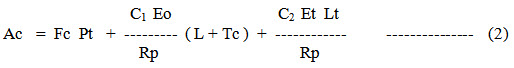
Therefore, annual costs of operating a tractor can be written as

Writing purchase price of tractor,       Pt  =   Rp  Pu

Where,

Pu        =          Price per unit power of tractor, Rs/kW

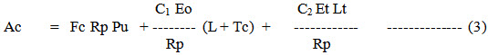
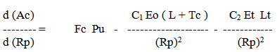
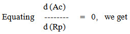
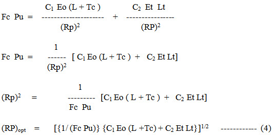
Differentiating the equation 10 with respect to Rp, we get

Differentiating equation 11 once again with respect to Rp, we get 

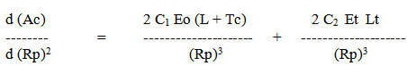
Which is a positive quantity, indicating that the calculated (R_P)_opt  would have a minimum cost of operation.

In equation (11), Eo in general can be rewritten as

Where,

i           = Subscript identifying specific operation, area, energy value etc.

A         = Area under crop, ha

E          = Energy required by a particular machine, kWh/ha

r           = Ratio of drawbar power to axle power

n          = number of passes of an implement

Energy required by a particular machine per unit area can be calculated by

Where,

E          = energy required by a particular machine per unit area, kWh/ha

P          = power required for operation, kW

Lc        = load coefficient factor

w         = width of implement, m

S          = speed of operation, km/h

E_f         = efficiency of machine

Timeliness of a field operation must be considered in selection of optimum power required of a tractor.  Timeliness costs arise because of the inability of a machine to complete a field operation in a reasonably short time. These are not out-of-pocket costs but reductions in potential returns as and when the yield and quality of crops are reduced because of delays in field operations. Delays due to bad weather cannot be charged to machine. Timeliness costs are so important that in a machinery selection process they must be evaluated quantitatively and considered as a valid cost of field machinery. In order to calculate this cost, the total reduction in returns is distributed over total hours of the actual use of tractor/machine. Total timeliness cost for an operation depends upon the scheduling of operations (delayed, premature and balance).  So, the total timeliness cost (Tc) can be estimated as:

                                                  K Y V A

                                    Tc   =   ---------------             --------------- (5) 

                                                  Sc Nt U h

Where,

Tc        =           Timeliness costs, Rs/h

K         =           Timeliness loss factor

Y         =           Crop yield, t/ha

V         =           Value of crop, Rs/t

A         =           Total area under crop, ha

U         =           Ratio of total working days to total days, fraction

Nt        =           Number of times area (A) should be divided because of dispersed optimum time

Sc        =           2 for premature or delayed scheduling

            =           4 for balanced scheduling

h          =          Actual number of hours utilized per day

Total timeliness costs for an operation depend on the scheduling of operations with respect to time and duration of operation.  There are basically three types of scheduling of operations viz. delayed, premature and balanced.  In delayed scheduling, operation starts at optimum time whereas in premature scheduling operation is completed by the optimum time.  In the balanced scheduling, operation is planned in such a way that it spreads over equally on both sides of the optimum time.  Therefore, time devoted in case of delayed and premature scheduling is half of that of balanced scheduling.  Thus, X is taken as 2 for premature or delayed and 4 for balanced scheduling.

The cost of untimely operations can be included in the basic cost model as a cost for each hour the machine is used.  The absolute costs depend on the value of the crop. Therefore, a relative timeliness factor called K has been developed to give some generality to the analysis (Table 3.6). K is defined as the decimal reduction of the quantity and quality of the potential crop per hour of machine operation.

Thus,

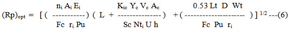
Where,

Fc        = Fixed cost percentage of a tractor

Pu       = Price per unit power of tractor, Rs/hp

A_i        = Area under crop, ha

E_i         = Energy required for operating an implement for a particular crop

K_ic       = Timeliness loss factor of an implement for a particular crop

Yc       = Yield of crop, q/ha

V_c        = Value of crop, Rs/q

U         =  Ratio of total working days to total days, fraction

Nt        =  Number of times area (A) should be divided because of dispersed optimum time

Sc        =  2 for premature or delayed scheduling

=  4 for balanced scheduling

h          =  Actual number of hours utilized per day

Lt        =  Labour rate for transportation, Rs/h

D         =  Distance to be travelled, km

Wt       =  Weight to be transported, tonne

r_i          = Ratio of drawbar power to rated engine power for drawbar

               load and ratio of PTO power to rated engine power for PTO

               loads for a particular crop

Note that repairs, fuel and oil costs have been dropped from considerations. Only labour and tractor fixed costs remain in the equation 13.  Equation 13 may be used without reservation for self-propelled implements and for selection of implements to fit into an existing machinery system where the tractor fixed costs are known and are constant. In fact, the optimum implement width may be more dependent upon the size of tractor than upon any of the other factors in equation 13.  Selection of an economic system of machines is highly dependent upon the horsepower level of the tractor or tractors.

Therefore, optimum tractor power required for drawbar operations can be calculated by

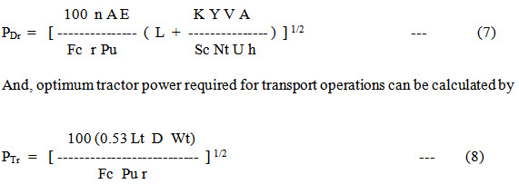
Total power required can be calculated by adding equations 14 and 15

i.e.   P  = P_Dr  + P_Tr

or

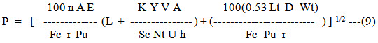
Overall power requirement would be sum of all the power requirements for specific operation of an implement for a particular crop and for all crops grown by the farmers. i.e.

Where,

i = subscript refers to specific operation of an implement

j = subscript refers to specific crop grown by the farmers

Table 1:  Timeliness loss factor for different operations and crops under Indian Farm conditions.

Crop	Operation	K value
Wheat	Tillage & sowing	0.00456
	Harvesting & threshing	0.00650
Barley	Tillage & sowing	0.0067
	Harvesting & threshing	0.0044
Paddy	Tillage & sowing	0.00625
	Harvesting & threshing	0.0066
Maize	Tillage & sowing	0.0046
Soybean	Tillage & sowing	0.0179
	Harvesting & threshing	0.0189
Moong	Tillage & sowing	0.0052
	Harvesting & threshing	0.066
Oil seeds	Tillage & sowing	0.0138
	Harvesting & threshing	0.035
Sunflower	Tillage & sowing	0.0035
	Harvesting & threshing	0.0035
Potato	Tillage & sowing	0.002
	Harvesting & threshing	0.002
Mash	Tillage & sowing	0.0052
	Harvesting & threshing	0.066
Gram	Tillage & sowing	0.0052
	Harvesting & threshing	0.066
Groundnut	Tillage & sowing	0.0138
	Harvesting & threshing	0.0351
Sugarcane	Tillage & sowing	0.002
	Harvesting & threshing	0.002
Cotton	Tillage & sowing	0.0138
	Harvesting & threshing	0.0351