Site pages
Current course
Participants
General
MODULE 1. Analysis of Statically Determinate Beams
MODULE 2. Analysis of Statically Indeterminate Beams
MODULE 3. Columns and Struts
MODULE 4. Riveted and Welded Connections
MODULE 5. Stability Analysis of Gravity Dams
Keywords
5 April - 11 April
12 April - 18 April
19 April - 25 April
26 April - 2 May
LESSON 6. Deflection of Beam: Conjugate Beam Theory
6.1 Introduction
A conjugate beam is a fictitious beam that corresponds to the real beam and loaded with M/EI diagram of the real beam. For instance consider a simply supported beam subjected to a uniformly distributed load as shown in Figure 5.1a. Figure 5.1b shows the bending moment diagram of the beam. Then the corresponding conjugate beam (Figure 5.1c) is a simply supported beam subjected to a distributed load equal to the M/EI diagram of the real beam.
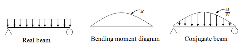
Fig. 6.1.
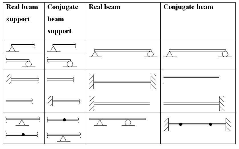
Supports of the conjugate beam may not necessarily be same as the real beam. Some examples of supports in real beam and their conjugate counterpart are given in Table 6.1.
Table 6.1: Real beam and it conjugate counterpart
Once the conjugate beam is formed, slope and deflection of the real beam may be obtained from the following relationship,
Slope on the real beam = Shear on the conjugate beam
Deflection on the real beam = Moment on the conjugate beam
6.2 Example 1
A cantilever beam AB is subjected to a concentrated load P at its tip as shown in Figure 6.2. Determine deflection and slope at B.
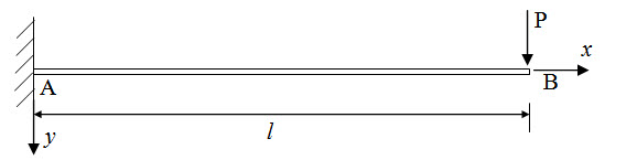
Fig. 6.2.
Solution
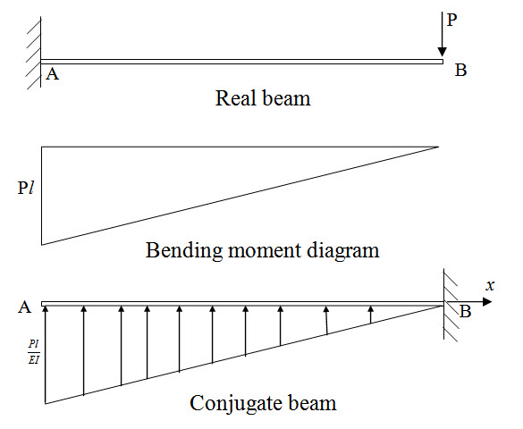
Fig. 6.2.
Real beam and corresponding conjugate beam are shown in Figure 6.2. Now, from the free body diagram of the entire structure (Figure 6.3), we have
\[{B_y}=-{1 \over 2}{{Pl} \over {EI}}l=-{{P{l^2}} \over {2EI}}\]
\[{M_B}={1 \over 2}{{Pl} \over {EI}}l{{2l} \over 3}={{P{l^3}} \over {3EI}}\]
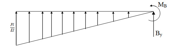
Fig. 6.3.
\[{\theta _B}={B_y}=-{{P{l^2}} \over {2EI}}\]
\[{\delta _B}={M_B}=-{{P{l^3}} \over {3EI}}\]
6.3 Example 2
A simply supported beam AB is subjected to a uniformly distributed load of intensity of q as shown in Figure 6.4. Calculate θA, θB and the deflection at the midspan. Flexural rigidity of the beam is EI.
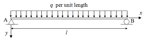
Fig. 6.4.
Solution
Bending moment and conjugate beam are shown in Figure 6.5.
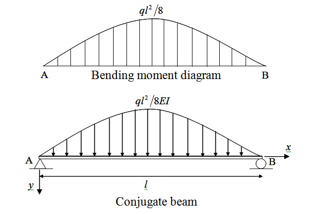
Fig. 6.5.
\[{A_y}={B_y}={1 \over 2} \times {\rm{Area of the parabolic load distribution }}\]
\[\Rightarrow {A_y} = {B_y}={1 \over 2} \times {2 \over 3}l{{q{l^2}} \over 8}={{q{l^3}} \over {24}}\]
Shear force of the conjugate beam at A and B are respectively as Ay and By.
Therefore,
\[{\theta _A}={A_y}={{q{l^3}} \over {24}}\] and \[{\theta _B}={B_y}={{q{l^3}} \over {24}}\]
Now in order to determine bending moment of the conjugate beam at the midspan the following free body diagram is considered.
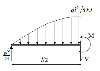 Fig. 6.6.
Applying equilibrium condition we have,
\[M={{q{l^3}} \over {24EI}}{l \over 2}-{{q{l^3}} \over {24EI}}{{3l} \over {16}}={{5q{l^4}} \over {384EI}}\]
Since deflection at the midspan of the real beam is equal to the bending moment at the midspan of the conjugate beam, we have,
\[\delta= M = {{5q{l^4}} \over {384EI}}\]
Suggested Readings
Hbbeler, R. C. (2002). Structural Analysis, Pearson Education (Singapore) Pte. Ltd.,Delhi.
Jain, A.K., Punmia, B.C., Jain, A.K., (2004). Theory of Structures. Twelfth Edition, Laxmi Publications.
Menon, D., (2008), Structural Analysis, Narosa Publishing House Pvt. Ltd., New Delhi.
Hsieh, Y.Y., (1987), Elementry Theory of Structures , Third Ddition, Prentrice Hall.
Last modified: Tuesday, 17 September 2013, 5:15 AM