Gulley & Ravine Control Structures 3(2+1)

Lesson 17 Estimation of Soil Erosion

17.2 The Universal Soil Loss Equation (USLE)

The USLE developed in the USA is the most widely used empirical model worldwide for estimating soil loss (Wischmeier and Smith, 1965). Information from the USLE is used in planning and designing conservation practices. This model is not strictly based on hydraulic principles and soil erosion theory.  It makes simplified assumptions in the processes of soil erosion. The USLE was specifically intended to predict soil loss from cultivated soils under specific characteristics.  It has sometimes been used inappropriately and applied to soil and land use conditions different from those for which it was developed. It provides a long-term annual average estimate of soil loss from small plots or field segments with defined dimensions. The USLE was developed from measured data rather than using physically-based modeling approaches.

The limited consideration of all the complex and interactive factors and processes of soil erosion with the USLE limits its applicability to all conditions.

The USLE is, however, advantageous over sophisticated models because it is simple, easy to use, and does not require numerous input parameters or extensive data sets for prediction. The simplicity of the equation for its practical use has sacrificed accounting for all the details of soil erosion.  Parameters are estimated from simple graphs and equations.  Unlike process-based models, the USLE cannot simulate the following:

• Runoff, nutrient, and soil loss from watersheds or large catchment areas.

• Soil loss on an event or daily basis and variability of soil loss from storm to storm.

• Interrill, rill, gully, and streambank erosion separately.

• Processes of concentrated flow or flow channelization and sediment deposition.

• Detailed processes (e.g., detachment, transport, and deposition).

The average annual soil loss is estimated as:

A= R*K*LS*C*P

Where, A is average annual soil loss (Mg ha⁻¹), R is rainfall and runoff erosivity index for the location of interest, K is erodibility factor, LS is topographic factor, C is cover and management factor, and P is support practice factor. The early versions of USLE were exclusively solved using tables and figures (e.g. nomographs). The continued improvement has resulted in MUSLE and Revised USLE (RUSLE 1and 2).

• Rainfall and Runoff Erosivity Index (EI)

The EI is computed as the product of total storm energy (E, J/m²) times the maximum 30-min intensity (I₃₀) of the rain (mm h^-1).

EI = E × I₃₀

The USLE uses the annual EI which is computed by adding the EI values from individual storms that occurred during the year. According to Wischmeier and Smith (1978), the EI corresponds closely to the amount of soil loss from a field. The EI as used in the USLE over-estimates the EI for tropical regions with intensive rains. The USLE-computed EI is only valid for rain intensities ≤ 63.5mm h⁻¹. Modifications to EI have been proposed for tropical regions (Lal, 1976). The 30-minute intensity for a given storm and location is obtained from rain gauge charts recording the rainfall. Values of EI₃₀ below 50 (mm h^-1) correspond to dry regions and those above 500 (mm h^-1) correspond to humid regions.

• Rainfall Erosivity factor (R)

The erosivity factor of rainfall (R) is a function of the falling raindrops and the rainfall intensity, Wischmeier and Smith (1958) found that the product of the kinetic energy (E, j/m²) of the raindrop and the maximum intensity of rainfall over a duration of 30 minutes (I₃₀) of the rain (mm h^-1), in a storm, was the best estimator of soil loss. This product is known as EI value.

EI = E × I₃₀                                                                  (17.2)

The USLE uses the annual EI which is computed by adding the EI values from individual storms that occurred during the year. According to Wischmeier and Smith (1978), the EI corresponds closely to the amount of soil loss from a field. The EI as used in the USLE over-estimates the EI for tropical regions with intensive rains. The USLE-computed EI is only valid for rain intensities ≤ 63.5mm h⁻1. Modifications to EI have been proposed for tropical regions (Lal, 1976). The 30-minute intensity for a given storm and location is obtained from rain gauge charts recording the rainfall. Values of EI30 below 50 (mm h^-1) correspond to dry regions and those above 500 (mm h^-1) correspond to humid regions.

• Soil Erodibility Factor (K)

Soil erodibility refers to soil’s susceptibility to erosion. It is affected by the inherent soil properties. The K values for the development of USLE were obtained by direct measurements of soil erosion from fallow and row-crop plots across a number of sites in the USA primarily under simulated rainfall. The K values are now typically obtained from a nomograph or the following equation:

K =  [0.00021 × M1.14 × (12 − a) + 3.25 × (b − 2) + 3.3 × 10−3(c − 3)] /100

M = (% silt + % very fine sand) × (100 − % clay)

Where, M is particle-size parameter, a is % of soil organic matter content, b is soil structure code (1 = very fine granular; 2 = fine granular; 3 = medium or coarse granular; 4 = blocky, platy, or massive), and c profile permeability (saturat d hydraulic conductivity) class [1 = rapid (150 mm h⁻¹); 2 = moderate to rapid (50–150 mm h⁻¹); 3 = moderate (12–50 mm h⁻¹); 4 = slow to moderate (5–15 mm h⁻¹); 5 = slow (1–5 mm h⁻¹); 6 = very slow (<1 mm h⁻¹)]. The size of soil particles for very fine sand fraction ranges between 0.05 and 0.10 mm, for silt content between 0.002 and 0.05, and clay <0.002 mm. The soil organic matter content is computed as the product of percent organic C and value given in Table 17.1.

Table 17.1.  K Factor Data (Organic Matter Content)

Textural Class	Average	Less than 2 %	More than 2 %
Clay	0.22	0.24	0.21
Clay Loam	0.30	0.33	0.28
Coarse Sandy Loam	0.07	--	0.07
Fine Sand	0.08	0.09	0.06
Fine Sandy Loam	0.18	0.22	0.17
Heavy Clay	0.17	0.19	0.15
Loam	0.30	0.34	0.26
Loamy Fine Sand	0.11	0.15	0.09
Loamy Sand	0.04	0.05	0.04
Loamy Very Fine Sand	0.39	0.44	0.25
Sand	0.02	0.03	0.01
Sandy Clay Loam	0.20	-	0.20
Sandy Loam	0.13	0.14	0.12
Silt Loam	0.38	0.41	0.37
Silty Clay	0.26	0.27	0.26
Silty Clay Loam	0.32	0.35	0.30
Very Fine Sand	0.43	0.46	0.37
Very Fine Sandy Loam	0.35	0.41	0.33

(Source: http://www.omafra.gov.on.ca/english/engineer/facts/00-001.htm#background)

• Topographic Factor (LS)

The USLE computes the LS factor as a ratio of soil loss from a soil of interest to

that from a standard USLE plot of 22.1m in length with 9% slope as follows:

LS = (Length/22.1)^m (65.41 sin² θ + 4.56 sin θ + 0.065)

m = 0.6 (1 − exp (−35.835 × S))

θ = tan⁻¹ (S/100)

Where, S is field slope (%) and θ is field slope steepness in degrees.

Table 17.2.  LS Factor Calculation

Slope Length ft (m)	Slope (%)	LS Factor
100 ft (31 m)	10	1.3800
	8	0.9964
	6	0.6742
	5	0.5362
	4	0.4004
	3	0.2965
	2	0.2008
	1	0.1290
	0	0.0693
200 ft (61 m)	10	1.9517
	8	1.4092
	6	0.9535
	5	0.7582
	4	0.5283
	3	0.3912
	2	0.2473
	1	0.1588
	0	0.0796
400 ft (122 m)	10	2.7602
	8	1.9928
	6	1.3484
	5	1.0723
	4	0.6971
	3	0.5162
	2	0.3044
	1	0.1955
	0	0.0915
800 ft (244 m)	10	3.9035
	8	2.8183
	6	1.9070
	5	1.5165
	4	0.9198
	3	0.6811
	2	0.3748
	1	0.2407
	0	0.1051
1600 ft (488 m)	10	5.5203
	8	3.9857
	6	2.6969
	5	2.1446
	4	1.2137
	3	0.8987
	2	0.4614
	1	0.2964
	0	0.1207
3200 ft (975 m)	10	7.8069
	8	5.6366
	6	3.8140
	5	3.0330
	4	1.6015
	3	1.1858
	2	0.5680
	1	0.3649
	0	0.1386

(Source: http://www.omafra.gov.on.ca/english/engineer/facts/12-051.htm)

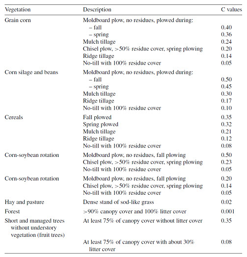
• Cover-Management Factor (C)

The C-factor is based on the concept that soil loss changes in response to the vegetative crop cover during the five crop stage periods: rough fallow, seedling, establishment, growing, and maturing crop, and residue or stubble. It is computed as the soil loss ratio from a field under a given crop stage period compared to the loss from a field under continuous and bare fallow conditions with up- and down-slope tillage (Wischmeier and Smith, 1978). Depending on the crop type and tillage method, the two sub-factors defining the C, are multiplied to compute the C-values. Estimates of C values for selected vegetation types are shown in Table 17.4. Detailed calculations of C values are presented by Wischmeier and Smith (1978).

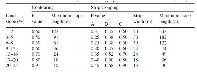
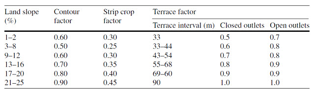
• Support Practice Factor (P)

The P-factor refers to the practices that are used to control erosion. It is defined as the ratio of soil lost from a field with support practices to that lost from a field under up-and down-slope tillage without these practices. The P values vary from 0 to 1 where the highest values correspond to a bare without any support practices. Maintaining living and dead vegetative cover and practicing conservation tillage significantly reduces soil erosion. The combined use of various practices is more effective than a single practice for controlling erosion in highly erodible soils. In such a case, support practices (P) including contouring, contour strip-cropping, terracing, and grass waterways must be used. The P values are obtained from Tables 17.4 and 17.5.

In systems with various support practices, P values are calculated as follows:

P = Pc × Ps × Pt      

where Pc is contouring factor for a given field slope, Ps is strip cropping factor, and Pt is terrace sedimentation factor (Table 17.5).

Table 17.3. “C” values for some tillage and cropping systems

 (Source: Humberto and Lal, 2008)

Table 17.4. P values for contouring and strip-cropping

(Source: Humberto and Lal, 2008)

Table 17.5.   P values for combined support practices

(Source: Humberto and Lal, 2008)

Table 17.6. Management Strategies to Reduce Soil Losses

Factor	Management Strategies	Example
R	The R Factor for a field cannot be altered.	--
K	The K Factor for a field cannot be altered.	--
LS	Terraces may be constructed to reduce the slope length resulting in lower soil losses.	Terracing requires additional investment  and will cause some inconvenience in farming. Investigate other soil conservation  practices first.
C	The selection of crop types and tillage methods that result in the lowest possible C  factor will result in less soil erosion.	Consider cropping systems that will provide maximum protection to the soil.  Use minimum tillage systems where possible.
P	The selection of a support practice that has the lowest possible factor associated with it  will result in lower soil losses.	Use support practices such as cross slope farming that will cause sediment deposition close to the source.

(Source: http://www.omafra.gov.on.ca/english/engineer/facts/05-067.htm)

17. 3 Application of USLE

1. The USLE was developed as a working tool for soil erosion prediction and soil conservation and erosion control planning. It was developed for application on very small land areas e.g. single fields within a farm, and most of the quantification of the factors in the equation were developed from studies on small field plots.

2. Application of the USLE to the analysis of nonpoint source pollution has been increasing in recent years and in many cases may be used beyond its limitations. Better predictive tools are needed, particularly with respect to sediment delivery ratios, and models which consider the physical processes involved in erosion and sediment transport.

3. The USLE only predicts soil loss by sheet and rill erosion as a result of rainfall impact on soils. The movement of dislodged soil particles to streams is not modelled. In some applications of the USLE, this is covered by a sediment delivery ratio (S_d). The determination and use of sediment delivery ratios is subject to considerable controversy and misuse.

17.4 Limitations of USLE

1. The model applies only to sheet erosion since the source of energy is rain; so it never applies to linear or mass erosion and predicts the average soil loss.

2. The type of countryside: the model has been tested and verified in plain and hilly countries with 1-20% slopes, and excludes young mountains, especially slopes steeper than 40%, where runoff is a greater source of energy than rain and where there are significant mass movements of earth.

3. The type of rainfall: the relations between kinetic energy and rainfall intensity generally used in this model apply only to the American Great Plains, and not to mountainous regions although different sub-models can be developed for the index of rainfall erosivity, R.

4. The model applies only for average data over 20 years and is not valid for individual storms. A MUSLE model has been developed for estimating the sediment load produced by each storm, which takes into account not only rainfall erosivity but also the volume of runoff (Williams 1975).

5. Lastly, a major limitation of the model is that it neglects certain interactions between factors in order to distinguish more easily the individual effect of each factor. For example, it does not take into account the effect on erosion of slope combined with plant cover, or the effect of soil type along with the effect of slope.

6. The USLE does not calculate sediment deposition.