Gulley & Ravine Control Structures 3(2+1)

Lesson 21 Models for Predicting Sediment Yield - II

21.2 The LISEM Model

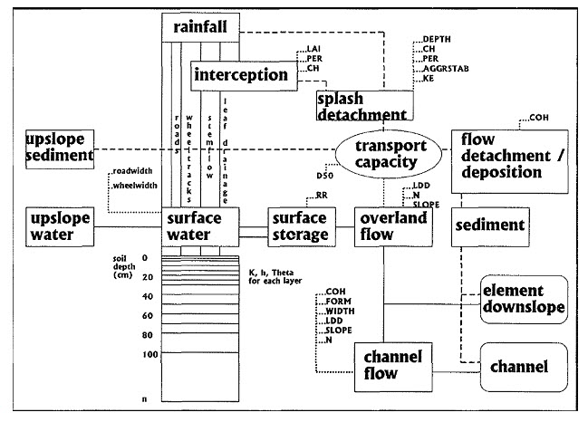
The Limburg Soil Erosion Model (LISEM) is a physically-based hydrological and soil erosion model, which can be used for planning and conservation purposes. LISEM simulates runoff and sediment transport in catchments caused by individual rainfall events. Processes incorporated in the model are rainfall, interception, surface storage in micro-depressions, infiltration, vertical movement of water in the soil, overland flow, channel flow, detachment by rainfall and throughfall, detachment by overland flow, and transport capacity of the flow. Also, the influence of tractor wheels, small paved roads (smaller than the pixel size) and surface sealing on the hydrological and soil erosion processes is taken into account. For infiltration and vertical transport of water in the soil, a LISEM user has the following options: (0) no infiltration; (1) Richards' equation for uniform soils; (2) Richards' equation for soils and wheel tracks; (3) Richards' equation for soils, wheel tracks and crusts; (4) Holtan; (5) one-layer Green-Ampt and (6) two-layer Green-Ampt. The Richards' equation is solved separately for uncrusted soils, crusted soils and wheel tracks. In areas without detailed knowledge of soil physics, the empirical Holtan/Overton infiltration equation (e.g. Beasley et al., 1980; De Roo, 1993b) can be used. However, the Holtan equation only simulates Hortonian overland flow; saturation overland flow is not simulated. Using the Richards-based sub-model, one can simulate overland flow. In other cases, the user may choose a one or two layer Green & Ampt model.

The major differences between LISEM and other erosion models are:

• on a GIS level LISEM uses a raster type representation of the catchment, such as in ANSWERS, which allows for a detailed representation of the processes. This is different from other process-based models such as EUROSEM or WEPP that use large polygon type elements;

• on a programming level LISEM is constructed with a specially designed spatial modeling language which allows for great flexibility (Fig. 21.1);

• on a process level LISEM comes conceptually close to EUROSEM and WEPP, while e.g. ANSWERS uses many empirical relationships. The possible use within LISEM of the SWATRE solution of the Richards' equation makes it more physically-based. The user also can choose Green and Ampt or the Holtan equation.

Fig. 21.1.  Processes involved in the LISEM Model. (Source: http://www.iahs.info/redbooks/a235/iahs_235_0395.pdf)

21.3 Erosion-Productivity Impact Calculator (EPIC)

The Erosion-Productivity Impact Calculator (EPIC) (Williams et al. 1984) model was originally developed to assess the effect of soil erosion on soil productivity. It was used for that purpose as part of the 1985 RCA (1977 Soil and Water Resources Conservation Act of USA) analysis. Since the RCA application, the model has been expanded and refined to allow simulation of many processes important in agricultural management.

EPIC is a continuous simulation model that can be used to determine the effect of management strategies on agricultural production and soil and water resources. The drainage area considered by EPIC is generally field-sized, up to 100 ha (247 ac) (weather, soils, and management systems are assumed to be homogeneous). The major components in EPIC are: weather simulation, hydrology, erosion sedimentation, nutrient cycling, pesticide fate, plant growth, soil temperature, tillage, economics, and plant environment control.

The EPIC component for water-induced erosion simulates erosion caused by rainfall and runoff and by irrigation (sprinkler and furrow). To simulate rainfall/ runoff erosion, EPIC contains six equations- the USLE (Wischmeier and Smith, 1978), the Onstad-Foster modification of the USLE (Onstad and Foster, 1975), the MUSLE (Williams, 1975), two recently developed variations of MUSLE, and a MUSLE structure that accepts input coefficients. Only one of the equations (user specified) interacts with other EPIC components. The six equations are identical except for their energy components. The USLE depends strictly upon rainfall as an indicator of erosive energy. The MUSLE and its variations use only runoff variables to simulate erosion and sediment yield. The Onstad-Foster equation contains a combination of the USLE and MUSLE energy factors. The original EPIC wind erosion model (WEQ) required daily mean wind speed as a driving variable. The new EPIC wind erosion model, Wind Erosion Continuous Simulation (WECS), requires the daily distribution of wind speed to take advantage of the more mechanistic erosion equation. The new approach estimates potential wind erosion for a smooth bare soil by integrating the erosion equation through a day using the wind speed distribution. Potential erosion is adjusted using four factors based on soil properties, surface roughness, cover, and distance across the field in the wind direction. The EPIC model with C0₂ capabilities has been used in several major studies in the United States.

21.4 Silt Yield Index Model

The Silt Yield Index (SYI) is defined as the Yield per unit area and SYI value for hydrologic unit is obtained by taking the weighted arithmetic mean over the entire area of the hydrologic unit by using suitable empirical equation. The Silt Yield Index Model developed by All India Soil & Land Use Survey (Dept of Agriculture, Govt. of India) was used for calculating sediment yield Index.

Estimation of Soil Loss Using Silt Yield Index (SYI) Method

The Silt Yield Index Model (SYI), considering sedimentation as product of erosivity, erodibility and areal extent was conceptualized in the All India Soil and Land Use Survey (AISLUS) as early as 1969 and has been in operational use since then to meet the requirements of prioritization of smaller hydrologic units. The erosivity determinants are the climatic factors and soil and land attributes that have direct or reciprocal bearing on the unit of the detached soil material.

The relationship can be expressed as:

Soil erosivity = f (Climate, physiography, slope, soil parameters, land use/land cover, soil management)

The erosivity is simulated with the sediment yield weightage value which is based on assessment of the composite effect of assemblage of erosivity determinants. Whereas, the delivery ratio is adjudged by the likely delivery of the eroded material into the reservoir.

Prioritization of Watersheds/Sub-watersheds:

The prioritizations of smaller hydrologic units within the vast catchments are based on the Silt Yield Indices (SYI) of the smaller units. The boundary values or range of SYI values for different priority categories are arrived at by studying the frequency distribution of SYI values and locating the suitable breaking points. The watersheds/sub-watersheds is subsequently rated into various categories corresponding to their respective SYI values.

The application of SYI model for prioritization of sub-watersheds in the catchment areas involves the evaluation of:

a) Climatic factors comprising total precipitation, its frequency and intensity,

b) Geomorphic factors comprising land forms, physiography, slope and drainage characteristics,

c) Surface cover factors governing the flow hydraulics and

d) Management factors.

The data on climatic factors can be obtained for different locations in the catchment area from the meteorological stations whereas field investigations are required for estimating the other attributes.

The various steps involved in the application of model are:

• Preparation of a framework of sub-watersheds through systematic delineation

• Rapid reconnaissance surveys on 1:50,000 scale leading to the generation of a map indicating erosion-intensity mapping units.

• Assignment of weightage values to various mapping units based on relative silt-yield potential.

• Computing Silt Yield Index for individual watersheds/sub watersheds.

• Grading of watersheds/sub-watersheds into very high, high medium, low and very low priority categories.  

The area of each of the mapping units is computed and silt yield indices of individual sub watersheds are calculated using the following equations:

a. Silt Yield Index

SYI = ( Σ (A_i x W_i ) x 100)/ A_w;

Where,

 i = 1 to n

Where,

A_i = Area of i^th unit (EIMU)

W_i = Weightage value of i^th mapping unit

n = No. of mapping units

A_w = Total area of sub-watershed.

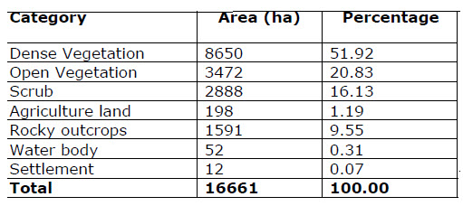
The SYI values for classification of various categories of erosion intensity rates are given in Table-21.1

Table 21.1. Land use pattern of a sample catchment area

Table 21.2. Criteria for erosion intensity rate priority categories

(Source:http://apspcb.org.in/pdf/28_12_10/NJC%20HEP%20REPORT-8.12.10/EMP%20Report%20Nyamjangchhu%20HEP_6.12.10/Chapter-2%20CAT%20Plan.pdf)

Any water resource project developer in India, such as irrigation project, hydro-electric project, etc. (private or government) is mandated by the Ministry of Environment and Forests to consider the very highly and highly eroded sub-watersheds (See Table 21.2) to bring under the purview of Catchment Area Treatment (CAT) Plan. A CAT plan usually comprises engineering and other measures for erosion control. The budget for CAT work in included in the project budget. The CAT is executed by the Forest Department of the state.

21.5 The ANSWER Model

Area Non-point source watershed environment response simulation (ANSWER) (Beasley and Huggins, 1982) uses a distributed parameter approach and is limited to a single storm event. Hydrology model components include rainfall interception, infiltration, surface detention and surface retention. A sediment continuity equation is employed which describes the process of soil detachment, transport and deposition. A watershed (up to 10,000 ha) being modeled is divided into a series of small independent element (1 to 4 ha). The use of small element allows considerable spatial details in representing topography, soils and land use but the building of input files and interpreting output requires significant time and considerable knowledge of the model and its operation.

21.6 SWAT Model

The Soil and Water Assessment Tool (SWAT) model was developed by US Department of Agriculture – Agriculture Research Service (USDA-ARS). It is a conceptual model that functions on a continuous time step. Model components include weather, hydrology, erosion/sedimentation, plant growth, nutrients, pesticides, agricultural management, channel routing, and pond/reservoir routing. Agricultural components in the model include fertilizer, crops, tillage options, and grazing and have the capability to include point source loads (Neitsch et al., 2001a; Neitsch et al., 2001b). The SWAT model predicts the influence of land management practices on constituent yields from a watershed. SWAT is the continuation of over 30 years of model development within the US Department of Agriculture’s Agricultural Research Service. SWAT is a public domain model which is actively supported by the USDA Agricultural Research Service at the Grassland, Soil, and Water Research Laboratory in Temple, Texas, USA.

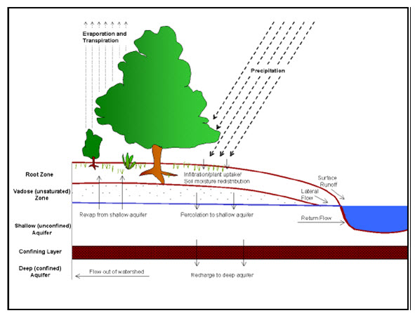
The SWAT model simulates hydrology as a two-component system, comprised of land hydrology and channel hydrology. The land portion of the hydrologic cycle is based on a water mass balance. Soil water balance is the primary considerations by the model in each HRU, which is represented as (Arnold et al., 1998):

SW_t = SW +∑ (R_i - Q_i - ET_i - P_i - QR_i)

Where,

SW is the soil water content, i is time in days for the simulation period t, and R, Q, ET, P and QR respectively are the daily precipitation, runoff, evapotranspiration, percolation, and return flow. Water enters the SWAT model’s watershed system boundary predominantly in the form of precipitation. Precipitation inputs for hydrologic calculations can either be measured data or simulated with the weather generator available in the SWAT model. Precipitation is partitioned into different water pathways depending on system characteristics. The water balance of each HRU in the watershed contains four storage volumes: snow, the soil profile (0-2 m), the shallow aquifer (2-20 m) and the deep aquifer (>20 m). The soil profile can contain several layers. The soil water processes include infiltration, percolation, evaporation, plant uptake, and lateral flow. Surface runoff is estimated using the SCS curve number or the Green-Ampt infiltration equation. Percolation is modeled with a layered storage routing technique combined with a crack flow model. Potential evaporation can be calculated using Hargreaves, Priestly-Taylor or Penman-Monteith method (Arnold et al., 1998).

Fig. 21.1. Hydrologic cycle considered by SWAT model. (Source: http://arkansaswater.org/materials/C%20SWAT%20Model%20Description%2004-20-2006.pdf)

21.7 MIKE SHE

MIKE SHE is a comprehensive, deterministic, distributed and physically based modeling system for the simulation of all major hydrological processes occurring in the land phase of the hydrological cycle. It simulates water flow, water quality and sediment transport. MIKE SHE comprises a number of comprehensive pre and post processors including digitizing, graphical editing, contouring, grid averaging and graphical result presentation with option for display of animation. Application of the model on PCs is limited because of the large number of computation that must be made.

MIKE SHE is applicable to a wide range of water resources and environmental problems related to surface water and groundwater system and the dynamic interaction between these. It is applicable on spatial scales from a single soil profile (infiltration studies) to large regions, which may include several river catchments.

21.8 HSPF Model

The hydrological simulation program-Fortran (HSPF) (Johansen et. al., 1984) is a mathematical model developed under EPA sponsorship to simulate hydrologic and water quality processes in natural and manmade water system. HSPF is a continuous simulation model and requires continuous data (generally hourly rainfall) to derive the simulations. This model requires input parameters for each of the various processes. Without calibration data, it can be difficult to verify the flows computed by this model.

Over the years, development activities and model enhancement, along with the model application, have continued to improve the model’s capabilities and preserve its status as a state-of-art-tool for watershed analysis.