Site pages
Current course
Participants
General
Module 1:Water Resources Utilization& Irrigati...
Module 2:Measurement of Irrigation Water
Module 3: Irrigation Water Conveyance Systems
Module 4: Land Grading Survey and Design
Module 5: Soil –Water – Atmosphere Plants Intera...
Module 6: Surface Irrigation Methods
Module 7: Pressurized Irrigation
Module 8: Economic Evaluation of Irrigation Projec...
Topic 9
LESSON 22. Infiltration
22.1 Infiltration Process
The process of entry of water into the soil is called infiltration, and the time rate at which water percolates into the soil is known as infiltration rate. Thus information about infiltration is needed for –
1) Hydrologic studies to determine runoff and percolation components
2) Designing irrigation systems
3) Managing of irrigation event, i.e., to determine water application rate and application time.
During the initial conditions when the soil is dry, the infiltration rate is high and decreases with time and tends to approach a constant rate (Fig. 22.1). This constant rate of infiltration is referred as the basic infiltration rate or final infiltration capacity or simply infiltration capacity of soil. The downward movement of infiltrated water through the soil profile is known as percolation. Accumulated infiltration or cumulative infiltration is the total quantity of water infiltrated into the soil in a given time. Fig. 22.1 shows both infiltration rate curve and accumulated or cumulative infiltration curve. Infiltration rate may change with respect to location, time/season and initial soil moisture content.
In water management and conservation studies, accurate information regarding the rate at which different soils will take water under different field conditions is required. The rate of entry of water into soil and the cumulative infiltration varies widely across different soil types and also within a single soil type, depending upon soil water content and management practices.
Why Infiltration Rate Decreases with Time?
-
The decrease in infiltration rate results from the decrease in the matric suction gradient (constituting one of the forces drawing water into the soil) which occurs as infiltration proceeds. If the surface of an initially dry soil is suddenly saturated, the matric gradient acting in the surface layer is at first very steep. As the wetted zone deepens, however, this gradient is reduced. Furthermore, as the thickness of the wetted soil increasesthe matric suction gradient eventually tends to become vanishingly small. Finally, infiltration rate reaches steady state condition.
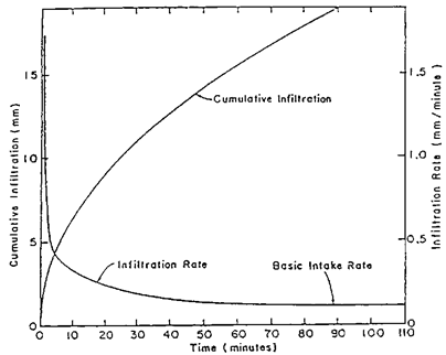
Fig.22.1. Plot of accumulated infiltration and average infiltration rate against elapsed time.(Source: www.scielo.br: accessed on May 28, 2013)
2. The decrease of infiltration rate from an initially high rate can in some cases result from gradual deterioration of soil structure, and consequent partial sealing of the profile by the formation of a dense surface crust or form the detachment and migration of pore-blocking particles or swelling of clay or air entrapment.
22.2 Infiltration Equations
Manyequations have been developed to represent the infiltration phenomena. Most of them are empiricalequations and have been developed to match observed data sets.One of the most commonly used infiltration equations particularly in the field of irrigation is the Kostiakov equation. It is described by the following equation:
Z = a t b (22.1)
and infiltration rate is given by,
I = ( a b ) tb-1 (22.2)
Where,
Z = depth of infiltration,cm
t = time or intake opportunity time, min
I = infiltration rate, cm/min, and
a and b= parameters (a > 0 and 0 <b< 1)
From Eq. (22.2), it is clear that as t → 0, I → ∞ and as t → ∞ , I → 0. In reality, infiltration rate, I, does not attain these values. However, because of the simplicity of the model it has been used widely in irrigation studies. Parameters of Eq (22.1) can be determined by plotting on log-log paper the accumulated infiltration Z against time and fitting a straight line.Similarly, parameters of Eq. (22.2) can also be determined.
log Z = log a + b log t (22.3)
Or log I = log (ab) + (b-1) log t (22.4)
Example 22.1:
A double ring infiltrometer test was conducted prior to an irrigation event and data recorded are given Table 21.1. Determine the parameters of the Kostiakov infiltration Equation (22.1).
Solution:
Take the log of time, t and as well as accumulated infiltration, Z. The log values are reported in Table 22.1. These log-log values are plotted and simple linear regression was performed, which resulted the following equation:
log Z = -0.502 + 0.773 log t
Taking the anti-log, the following equation results
Z = 0.315 log t(0.773)
|
Time, t |
Cum. Infil., Z |
log(t) |
log(Z) |
Predicted, Z |
|
(min) |
(cm) |
|
|
(cm) |
|
3 |
0.85 |
0.477 |
-0.071 |
0.736 |
|
5 |
1.12 |
0.699 |
0.049 |
1.093 |
|
10 |
1.77 |
1 |
0.248 |
1.868 |
|
15 |
2.44 |
1.176 |
0.387 |
2.555 |
|
20 |
3.07 |
1.301 |
0.487 |
3.191 |
|
25 |
3.63 |
1.398 |
0.56 |
3.792 |
|
30 |
4.18 |
1.477 |
0.621 |
4.366 |
|
35 |
4.73 |
1.544 |
0.675 |
4.919 |
|
40 |
5.26 |
1.602 |
0.721 |
5.454 |
|
45 |
5.8 |
1.653 |
0.763 |
5.973 |
|
50 |
6.34 |
1.699 |
0.802 |
6.48 |
|
55 |
6.83 |
1.74 |
0.834 |
6.976 |
|
60 |
7.31 |
1.778 |
0.864 |
7.461 |
|
65 |
7.82 |
1.813 |
0.893 |
7.937 |
|
70 |
8.3 |
1.845 |
0.919 |
8.405 |
|
75 |
8.79 |
1.875 |
0.944 |
8.866 |
|
80 |
9.27 |
1.903 |
0.967 |
9.319 |
|
85 |
9.78 |
1.929 |
0.99 |
9.766 |
|
90 |
10.26 |
1.954 |
1.011 |
10.208 |
|
95 |
10.7 |
1.978 |
1.029 |
10.643 |
|
100 |
11.2 |
2 |
1.049 |
11.074 |
|
105 |
11.67 |
2.021 |
1.067 |
11.499 |
|
110 |
12.16 |
2.041 |
1.085 |
11.92 |
|
115 |
12.62 |
2.061 |
1.101 |
12.337 |
|
120 |
13.09 |
2.079 |
1.117 |
12.75 |
|
125 |
13.59 |
2.097 |
1.133 |
13.158 |
|
130 |
14.02 |
2.114 |
1.147 |
13.563 |
|
135 |
14.48 |
2.13 |
1.161 |
13.965 |
|
140 |
14.98 |
2.146 |
1.176 |
14.363 |
Fig. 22.2 shows the comparison between the observed and predicted cumulative infiltration.
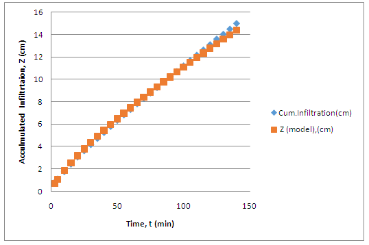
Fig. 22.2. Comparison between observed and predicted accumulated infiltration using the Kostiakov model.
To overcome the restrictions of original Kostikov infiltration equation, it was modified to include steady state infiltration term. The Modified Kostiakov Equation is given by
Z = a tb + c . t (22.4)
I = ( ab ) tb-1 + C (22.5)
Where a and b are the parameters and c is the steady state infiltration rate. The steady infiltration rate can be determined from infiltration measurements, when infiltration rate approaches near steady-state condition.
22.3Measurement of Infiltration
Infiltration rates are measured in a number of different ways. Out of several methods three which are commonly used are:
a) The use of double ring or cylinder infiltrometer (Fig 22.3)
b) Measurement of subsidence of free water in a large basin
c) Estimation of water front advance data
Infiltration rates for border type, and sometimes furrow type, irrigation systemsare commonly measured with a single-ring or double-ring type infiltrometer. Fig. 22.3 shows double ring infiltrometer.
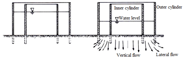
Fig.22.3. Section view of double-ring infiltrometer.
View at left is at t = 0 andview at right is after infiltration has proceeded for some time.
The cylinders are usually 25 cm deep and are formed of 2 mm rolled steel. The measurements are taken in inner cylinder having diameter of 30 cm. The outer cylinder, having 60 cm diameter, is used to create a buffer zone to reduce the lateral flow of water from the inner one. The cylinders are installed 10 cm deep in the soil. The water level in the inner cylinder is measured with a point gauge or ordinary scale installed inside the cylinder. The change in water level is measured with respect to time using a stop watch until the infiltration rate reached steady state (basic infiltration rate).
22.4 Factors Affecting Infiltration
The major factors influencing the infiltration include initial soil moisture content, soil surface conditions, hydraulic conductivity of the soil profile, texture, porosity, degree of swelling of soil colloids, organic matter, and vegetative cover, duration of irrigation or rainfall and viscosity of water. Initial moisture content has direct effect on infiltration rate and total amount of infiltration. Infiltration decreases with increase in initial soil moisture content. Infiltration rate or total infiltration increases as permeabilityand porosity increases. Cultivation increases the infiltration by improving the porosity. Infiltration rates are normally lower in heavy textured soils than in light textured soils (Figs. 22.4 and 22.5). Vegetation improves the infiltration of soil.
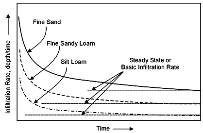
Fig.22.4. Rate of infiltration as an irrigation proceeds andthe steady rate of
Infiltration for three soil textures.(Source: Okstate.edu: accessed on May 28, 2013)
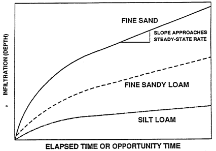
Fig. 22.5. Cumulative infiltration for three soil textures.(Source: Okstate.edu: accessed on May 28, 2013.)
Finally, it may be noted that infiltration characteristics of soils are highly vary both in space as well as in irrigation season. This is implies that there is need to evaluate infiltration characteristics at multiple sites as well as during crop season to obtain representative values of infiltration. Such information will be helpful to both designing and managing irrigation systems.
References
Michael, A.M. (2008). Irrigation Theory and Practice. Vikas Publishing House PvtLtd. New Delhi.
Murty, V.V.N. (2002).Land and Water Management Engineering (FourthEdition).Kalyani Publisher, New Delhi.
Internet References
http://www.angrau.ac.in/media/7380/agro201.pdf
http://gilley.tamu.edu/BAEN464/Handout%20Items/Cuenca%20Book%20Chapter%203%20Soil%20Physics.pdf
http://ilri.org/InfoServ/Webpub/fulldocs/IWMI_IPMSmodules/Module_3.pdf
ftp://ftp.wcc.nrcs.usda.gov/wntsc/waterMgt/irrigation/NEH15/ch1.pdf
Suggested Reading
http://www.fao.org/docrep/r4082e/r4082e03.htm
ftp://ftp.wcc.nrcs.usda.gov/wntsc/waterMgt/irrigation/NEH15/ch1.pdf
http://storm.okstate.edu/bae3313/Lecture/8)%20soilwaterplant%20relationships/soil-water-plant%20relationships.pdf
http://www.angrau.ac.in/media/7380/agro201.pdf
Last modified: Saturday, 15 March 2014, 6:12 AM