Irrigation Engineering 4(3+1)

LESSON 27. Irrigation Scheduling

In many cases irrigation scheduling is performed based on the irrigator's personal experience, plant appearance, watching the neighbor, or just simply irrigating whenever water is available. However, over the year a number of irrigation scheduling techniques based on soil water monitoring, plant monitoring and water balance approach have been developed.  Soil water monitoring techniques are already covered.  We will summarize these methods in this lecture but will focus on irrigation scheduling based on soil water balance approach.  Each of these irrigation scheduling philosophies have some shortcomings. To overcome these in the future a combination of soil water monitoring and plant status will be the most appropriate choice.

 

27.1.1 Advantages of Irrigation Scheduling

Irrigation scheduling offers several advantages:

1. It enables the farmer to schedule water rotation among the various fields to minimize crop water stress and maximize yields.
2. It reduces the farmer's cost of water and labouras it minimizes thenumber of irrigations.
3. It lowers fertilizer costs by holding surface runoff and deep percolation (leaching) to a minimum.
4. It increases net returns by increasing crop yields and crop quality.
5. It minimizes water-logging problems by reducing the drainage requirements.
6. It assists in controlling root zone salinity problems through controlled leaching.
7. It results in additional returns by using the "saved" water to irrigate non-cash crops that otherwise would not be irrigated during water-stress periods.

 

27.1.2 Full Irrigation

It provides the enough water to meet the entire irrigation requirement and is aimed at achieving the maximum production potential of the crop. Excess irrigation may reduce crop yield because of decreased soil aeration.

 

27.1.3 Deficit Irrigation

It means partially meeting the crop water requirement. It is practiced when there is water scarcity or the irrigation system capacity is limited. With deficit irrigation root zone is not filled to the field capacity moisture level.Deficit irrigation is justified in case where reducing water application below full irrigation causes production cost to decrease faster than revenue decline due to reduced yield. This method allows plant tress during one or more periods of growing season. However, adequate water is applied during the critical growth stages to maximize water use efficiency. Critical growth stage of some the crops are shown in the following Table 27.1.

 

Table 27.1.Critical growth stages for managing water use efficiency

Crop	Growth period Most sensitive to water  Stress	Growth Interval in which irrigation Produces Greatest Benefits
Sorghum	Boot- heading	Boot- soft dough
Wheat	Boot- flowering	Jointing- soft dough
Corn	Tassel- pollution	12 leaf- blister kernel
Cotton	First bloom- peak bloom	First bloom- boils well- formed
Dry beans	Flowering –early  podfill	Axillary bud- podfill
Potatoes	Tuberization	Tuberization- maturity
Soybean	Flowering- early podfill	Axillary bud- podfill
Sugarbeets	No critical stages	WUEa is maximized when water depletion is limited ton about 50% available water depletion

(Source: James, 1988)

 

27.1.4 Irrigation Interval

It is the number of days between two successive irrigations. It depends on the crop ET, effective rainfall, and available water holding capacity of the soil in the crop root zone and management allowable depletion.    

27.2 Methods of Irrigation Scheduling

Over the years, a number of methods have been developed for irrigation scheduling. These can be broadly classified into following categories:

1. Soil indicators

2. Climatological

3. Plant indices

4. Water balance

 

27.2.1 Soil Indicator

There are number of methods based on soil indicators. These include feel and appearance, soil moisture monitoring using gravimetric method, neutron probe, TDR, or soil moisture tension measurement using tensiometer, porous block etc. Soil moisture as well as soil moisture tension measurement is already discussed in previously. In these methods, the available soil water held between field capacity and permanent wilting point in the effective crop root zone depth is taken as guide for determining practical irrigation schedules. Alternatively soil moisture tension is also used as a guide for timing irrigations. Feel and appearance is one of the oldest and simple methods of determining the soil moisture content. It is done by visual observation and feel of the soil by hand. The accuracy of judgment improves with experience.

 

27.2.2 Climatological Approach (IW: CPE Ratio)

Irrigation scheduling on the basis of ratio betweenthe depth of irrigation water (IW) and cumulative evaporation from U.S.W.B. Class A panevaporimeter minus the precipitation since the previous irrigation (CPE) proposed by Prihar et al. (1974). The accuracy of the method depends on proper installation of pan evaporimeter and raingauge and the measurements of pan evaporation and rainfall.  Further, suitability of the method is site specific and limited to particular variety of crop.  An IW/CPE ratioof 1.0 indicates irrigating the crop with water equal to that lost in evaporation from theevaporimeter. A few examples of optimal IW/CPE ratios for important crops are given inTable 27.2.

 

Table 27.2. Optimum IW/CPE ratios for scheduling irrigation in important crops

Crop	Optimum IW/CPE ratio
Groundnut	♦	0.75 to 1.0 IW/CPE ratio depending on crop developmental stages in Andhra Pradesh, Maharashtra & West Bengal
Sunflower	♦	0.5 to 1.0 IW/CPE ratio depending on crop developmental stages at Hyderabad & Kanpur
Wheat	♦	1.0 IW/CPE ratio at Ludhiana, Kanpur and Bikramganj
Bengal gram	♦	0.4 IW/CPE ratio at Ludhiana
Mustard	♦	0.4 IW/CPE ratio at Hissar
Maize	♦	0.75 to 1.0 IW/CPE ratio depending on crop developmental stages at Delhi & Hyderabad
Sugarcane	♦	0.5 to 1.0 IW/CPE ratio depending on crop developmental stages at Lucknow

(Source: http://www.angrau.ac.in/media/7380/agro201.pdf: accessed on June 3, 2013)

 

27.2.3 Plant Indices Approach

The plants readily respond to the deficit in soil water. Some of the indices used to schedule irrigation based on this response are discussed below:

 

27.2.3.1 Visual Plant Symptoms

The visual signs of plants are used as an index for schedulingirritations. These include colour of plants, curling and rolling of leaves, wilting of leaves, change in leaf angle etc. Plant water stress in maize and beans crop is reflected throughrolling of leaves in case of maize and change in angle of leaves in case of bean (Fig. 27.2).  Successful interpretation of crop stress requires keen observation and experience. Secondly sometimes symptoms may be misleading and by the time they appear it may be too late to irrigate.

 

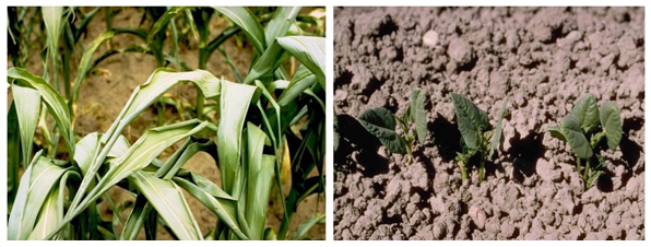
Fig. 27.3.Rolling of leaves in maize and change of leaf angle in beans.

(Source: http://www.angrau.ac.in/media/7380/agro201.pdf: accessed on June 3, 2013)

 

27.2.3.2 Plant Water Potential

Plant water potential is a measure of the energy status of plant water and is analogous to the energy measurements of soil water.This serves as a better index of physiological and bio-chemicalphenomena occurring in the plant. Plant or leaf water potential can be precisely measuredeither by a Pressure bomb or pressure chamber apparatus (figure. 27.4) are generally used for in situ measurement of leaf water potential, whereas the dye method is used in the laboratory. The critical plant water potential varies with crop. When potential values falls below critical limits specific to crop and growth stage, physiological and growth factors are adversely affected and thus they can serves as a guideline for irrigation scheduling.  In case of cotton critical potential ranges from 1.2 to 1.25 MPa throughout the crop life, whereas for sunflower they are 1.0, 1.2 and 1.4 MPa at vegetative, pollination and seed formation, respectively.

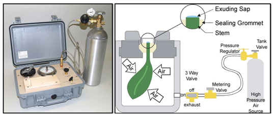
Fig. 27.4.Pressure chamber apparatus.

(Source: http://www.angrau.ac.in/media/7380/agro201.pdf: accessed on June 3, 2013)

 

27.2.3.3 Canopy Temperature

The canopy temperature reflects the internal water balance of the plant, and can be used as a potentialindicator for scheduling irrigation to crops. It can be measured by porometer, infrared thermometer (Fig 27.5) etc.The leaf canopy temperature is sensitive index in crops like soyabean, oats, barley, wheat, sorghum and maize.

 

Fig. 27.5.Infrared thermometer for scheduling irrigations to crops.

(Source: http://www.angrau.ac.in/media/7380/agro201.pdf: accessed on June 3, 2013)

 

27.2.4 Water Balance Approach

Irrigation scheduling based on water balance approach uses readily available information on weather, crop and soil information.  The soil water balance can be expressed in terms of soil moisture depletion as follows:

                  (27.1)

where SMD= total soil moisture depletion in the root zone and is defined as the difference between total soil moisture stored in the root zone at the field capacity and the current moisture status; ET_c = crop evapotranspiration; DP = deep percolation; I = irrigation amount; P_e= effective rainfall; GW = the capillary rise/ground water contribution and i = time index.

 

The initial soil moisture depletion at the beginning of the water balance or can be either assumed at field capacity or determined using the measured value of moisture content as follows:

                        (27.2)

 Where, D_rz = effective root zone depth, which increases during the growing season and reaches a maximum depth, = volumetric moisture content at field capacity and = initial volumetric moisture content.

 Daily crop evapotranspiration can be calculated as:

 

                    (27.3)                                      

WhereETo= grass reference crop ET and can be estimated using the methods discussed previously; K_c = crop coefficient which is a function of the crop type and the growth stage; K_s = crop stress coefficient which is a function of the soil moisture available to the crop.

 

Crop stress coefficient varies with moisture content as shown in Fig. 24.2. It can be estimated as follows for soil moisture depletion greater than readily available water (SMD_i> RAW):

                (27.4)

 K_s,i = 0                                                                 

SMD_i<RAW               (27.5)

 

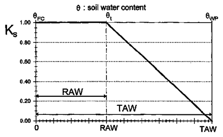
Fig. 24.2.Crop stress coefficient variation with moisture content. (Source: FAO 56)

Deep percolation from the root zone occurs when excess water from rain or irrigation fills the root zone beyond field capacity. It can be assumed that soil water content returns to the field capacity within the same day of wetting event. The deep percolation can be determined as follows:

                (27.6)

 

The deep percolation is zero (DP_i = 0), when irrigation and effective rainfall are less than or equal to SMD and ET_c.

Effective rainfall can be considered as some fixed percentage of rainfall and capillary rise can be neglected if water table is far below root zone. After evaluating each term of Eq. (27.1), irrigation scheduling can be performed based on fixed interval, fixed depth or management allowable depletion (MAD) criteria.

• For fixed interval, the estimated irrigation requirement is equal to soil moisture depletion at the end of the interval,

• For fixed depth case, irrigation is required when soil moisture depletion becomes equal to irrigation depth.

• In the case of irrigation scheduling based on MAD, both day of irrigation and depth are estimated as follows:
  

                                  (27.7)

Where AD = allowable depletion, MAD = management allowable depletion limit, defined as the fraction of TAW that can be safely removed from the soil to meet the daily ET demand on day i. In this case irrigation is given on the day i, when the soil moisture depletion reaches the allowable depletion. The required irrigation depth is equal to soil moisture depletion.

 

NRCS (1997) reported that MAD should be evaluated according to crop needs, and, if needed, adjusted during the growing season. Values of MAD, during the growing season are typically 25 to 40 percent for high value, shallow rooted crops; 50 percent for deep rooted crops; and 60 to 65 percent for low value deep rooted crops. Recommended MAD values by soil texture for deep rooted crops are:

• Fine texture (clayey) soils 40%

• Medium texture (loamy) soils 50%

• Coarse texture (sandy) soils 60%

 

Note that in all the cases, irrigation depth calculated is net irrigation depth and in order to determine gross application depth leaching requirement and application efficiency need to be taken into consideration. However, in many field conditions leaching requirement is need not to be considered for each irrigation.

Example 27.1:

For a crop with effective rooting depth of 150 cm, calculate the irrigation interval. Given, field capacity = 14%, permissible depletion 7 %, and crop evapotranspiration = 285 mm/ month.

 

Solution:

          Irrigation interval   =11.05 = 11 days

 

Example 27.2:

In the above problem, if during the period under consideration there is an effective rainfall of 35 mm, the irrigation interval will be,

 

Irrigation interval =  =14 days

 

Example 27.3:

A bean crop is grown in clay loam soil and is completely developed. The groundwater table is more than 5 m below the surface. At the beginning of mid season stage of crop, the moisture content is at field capacity. Reference crop evapotranspiration and precipitation values for the 10 day period are given below. 

 

Day	1	2	3	4	5	6	7	8	9	10
ETo mm/d	5.6	5.4	5.9	5.8	5.6	5.8	5.9	5.8	5.2	5.4
P, mm/d	0	0	0	0	5	0	0.2	0	0	0

 

Furthermore, consider effective root zone depth as 60 cm, crop coefficient as Kc_mid 1.05, volumetric water content at field capacity and permanent wilting points as 36% and 18%, respectively. Using the above information develop irrigation schedule based on a fixed interval of a week and MAD.

 

Solution:

Effective root zone depth = 60 cm, Kc_mid = 1.05,  = 36%,  = 18%  and MAD = 0.5 (based on soil)

Total available water, TAW = (Θ_fc - Θ_pwp ). D_rz = (0.36 - 0.18) (60) = 10.80 cm

Allowable depletion, AD = MAD .TAW = (0.5)(10.80) = 5.4 cm = 54 mm

 

At the beginning soil moisture is at field capacity and thus SMD_i-1 = 0. Calculation for each day is shown below:

Day	SMDi-1	EToi	Kci	Ksi	ETci	DPi	Ii	Pei	SMDi
	(mm)	(mm)			(mm)	(mm)	(mm)	(mm)	(mm)
1	0.0	5.6	1.05	1.0	5.9	0.0	0.0	0.0	5.9
2	5.9	5.4	1.05	1.0	5.7	0.0	0.0		11.6
3	11.6	5.9	1.05	1.0	6.2	0.0	0.0		17.7
4	17.7	5.8	1.05	1.0	6.1	0.0	0.0		23.8
5	23.8	5.6	1.05	1.0	5.9	0.0	0.0	5.0	24.7
6	24.7	5.8	1.05	1.0	6.1	0.0	0.0		30.8
7	30.8	5.9	1.05	1.0	6.2	0.0	0.0	0.2	36.8
8	36.8	5.8	1.05	1.0	6.1	0.0	0.0		42.9
9	42.9	5.2	1.05	1.0	6.0	0.0	0.0		48.4
10	48.9	5.4	1.05	1.0	6.2	0.0	0.0		54.0

 

For MAD based scheduling, 54.0 mm of irrigation would be required on the morning of 11^th day, whereas irrigation amount would be 36.8 mm after a week. 

 

References

Allen, R. G., Pereira, L. S., Raes, D., and Smith M. (1998). “Crop evapotranspiration: Guidelines for computing crop water requirements.” Irrigation and Drainage Paper No. 56. Rome: FAO.

James, L. G. (1988).  Principles of Farm Irrigation System Design. John Wiley & Sons, NY.

Michael, A.M. (2008). Irrigation Theory and Practice.Vikas Publishing House PvtLtd. New Delhi.

NRCS (1997).National Engineering Handbook, 652.USDA, Washington DC.

Murty, V.V.N. (2002).Land and Water Management Engineering (FourthEdition). Kalyani Publisher, New Delhi.

 

Internet References

http://www.angrau.ac.in/media/7380/agro201.pdf

http://gilley.tamu.edu/BAEN464/Handout%20Items/Cuenca%20Book%20Chapter%203%20Soil%20Physics.pdf

http://www.fao.org/docrep/r4082e/r4082e03.htm

http://ilri.org/InfoServ/Webpub/fulldocs/IWMI_IPMSmodules/Module_3.pdf

ftp://ftp.wcc.nrcs.usda.gov/wntsc/waterMgt/irrigation/NEH15/ch1.pdf

 

Suggested Reading

http://www.fao.org/docrep/r4082e/r4082e03.htm

ftp://ftp.wcc.nrcs.usda.gov/wntsc/waterMgt/irrigation/NEH15/ch1.pdf

http://storm.okstate.edu/bae3313/Lecture/8)%20soilwaterplant%20relationships/soil-water-plant%20relationships.pdf

http://www.academia.edu/705434/Comparison_of_techniques_for_measuring_he_water_content_of_soil_and_other_porous_media

http://www.angrau.ac.in/media/7380/agro201.pdf