Irrigation Engineering 4(3+1)

LESSON 23 Soil Water Movement

 

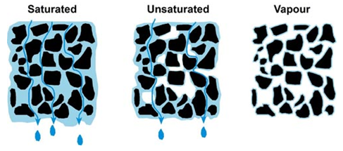
Fig. 23.1.Different types of soil water movement.

(Source:http://www.terragis.bees.unsw.edu.au/terraGIS_soil/images/water_fig_9.jpg: accessed on May 29, 2013)

23.2 Soil Water Movement in Saturated Condition

Under saturated condition of soil, all the macro and micro pores are filled with waterand any water flow under this condition is referredto as saturated flow.The saturated flow of water depends upon twofactors namely hydraulic gradient i.e., the hydraulic force driving the water through the soil andhydraulic conductivity i.e., the ease with which the soil pores permit water movement.

Assuming the soil to be a bundle of straight and smooth tubes, knowledge of the size distribution of the tube radii could enable us to calculate the total flow through a bundle caused by known pressure difference, using Poiseuille’s equation:

         (23.1)

 

Where,        q = volume of flow per unit time cm³/sec

P= pressure difference between two ends of the tube of length l, dynes/cm²

r = radius of the tube, cm

l = length of the tube, cm

μ = viscosity of liquid, dynes-sec/m²

The above equation indicates that the pore size is of outstanding significance, as its fourth power is proportional to the rate of saturated flow. Generally the rate of flow follows:

                                                Sand > Loam > Clay

Unfortunately, soil pores are not like straight tubes, but are of varying shapes and sizes, highly irregular and interconnected. This complexity in shape causes change in fluid velocity from point to point, even along the passage. For this reason, flow through complex porous media is generally described in terms of macroscopic flow velocity vector, which is the overall average of the microscopic velocities over a total volume of soil. Thequantity of water flowing through a section of saturated soil per unit of time isgiven by the Darcy’s law. Fig. 23.2 show typical setup for Darcy’s Law.

 

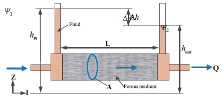
Fig. 23.2 Definition sketch of Darcy’s Law.

(Source: http://doi.ieeecomputersociety.org)

 

The law states that, the quantity of water passing through a unit cross sectional area of soil is directly proportional to the hydraulic gradient. Mathematically,

     (23.2)

(23.3)

Where,        Q    = volume flow cm³

q     = volume of flow per unit time cm³/sec

t      = time, sec

A= cross-sectional area of the soil through which the water flows, cm²

K_sat= saturated hydraulic conductivity, cm/sec

 Δh = change in water potential between the endsof the column, cm

 

(forexample, ₁ - ₂ )

L  = the length of column, cm

i= , hydraulic gradient.

V = velocity of flow cm/sec or velocity flux, v. It is the flow per unit area.

The negative sign denotes that the direction of flow is opposite to that of the head causing the flow. It is omitted in further discussions as its significance lies only in indicating the direction which is the same (towards the decreasing gradient) in all cases.

Darcy’s law is valid only when flow is laminar. Reynold’s number, the index used for describing the nature of flow is given by

 

            (23.4)

 

Where,        Re = Reynold’s number

 = density of fluid

                   V=velocity of flow

                   D = mean diameter of the soil particles

                   μ= dynamic viscosity of the fluid.

 

The Darcy’s law is valid for flows where Re is less than one.

In equation 23.3 the replacing Δμ  by Δψ  and we get

  (23.5)

Where, Δψ  = is the change in potential between two points at a distance l.

Application of Darcy’s law and continuity equation of three dimensional flow of an incompressible fluid through a porous medium results in the derivation of Laplace equation. It is given by

         (23.6)

It states that the second partial derivatives of the water potential with respect to x,y and z directions sums to zero.

23.3 Unsaturated Water Movement

As gravity drainage continues the soil macrospores emptied and aremostly filled up with air and the micro pores or capillary pores with water and some air. Movement of wateroccurring under this condition is termed as the unsaturated flow condition. In the case of unsaturated flow condition, the water potential is the sum of metric potential ( ψm) and gravitational potential (ψg) . Metric potential is only applicable in the case of horizontal movement of water. In the case of downward movement of water, capillary and gravitational potential act together. In the case of upward capillary movement of water, metric potential and gravitational potential oppose one another.For unsaturated flow condition of water through soil, equation 23.5 can be modified as:

           (23.7)

Darcy’s law can be applied in the case of unsaturated flow conditions with some modifications.

Unsaturated, 1-D horizontal flow is given by

        (23.8)

Unsaturated, 1-D vertical flow is given by

         (23.9)

 

Where K is hydraulic conductivity and D is diffusivity.

 

23.4 Hydraulic Conductivity

The hydraulic conductivity of a soil is the ability of soil to transmitwater when subjected to a hydraulic gradient. Hydraulic conductivity is defined by Darcy'slaw Eq. (23.3).

 

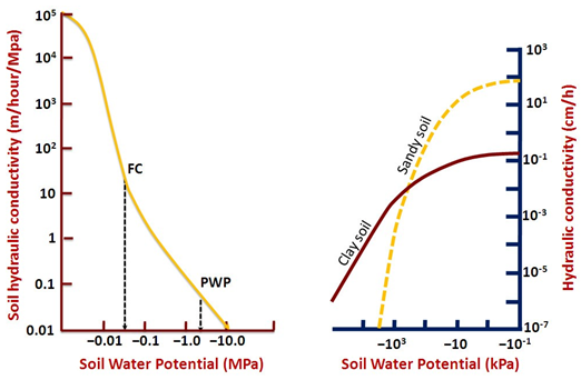
Fig. 23.3.Soil hydraulic conductivity versus soil water potential. (Source: Rao et. al, 2010)

 

The hydraulic conductivity is defined as the ratio of Darcy's flow velocity atunit hydraulic gradient.  K has a dimension of length per unit of time (L/T) which is same as that for velocity. The hydraulic conductivity is moreor less constant in a soil having a stable structure, however, it changes as the soil structure, density and porosity change. With variation in soil texture the hydraulic conductivity valuesare different. Typical values of saturated Hydraulic conductivity for different soil texture are given in Table 23.1.

 

Table 23.1. Saturated hydraulic conductivity for different soil textures

Soil class	Hydraulic conductivity, K (mm/hr)	Soil class	Hydraulic conductivity, K  (mm/hr)
Sand	50 (25-250)	Clay loam	8 (3-15)
Sandy loam	25 (12-75)	Silty clay	3 (0.25-5)
Loam	12 (8-20)	Clay	5 (1-10)

(Source: Hansen et al., 1979)

 

Clay soil with a large proportion of fine pores shows poor hydraulic conductivity as compared to a sandy soil with higher proportion of larger pores(Fig. 23.3). Higher bulk density and massive structure reduce the hydraulic conductivity ofthe soil. Saturated hydraulic conductivity for a particular soil is always constant, whereasunsaturated hydraulic conductivity is a function of soil water content.

 

23.4.1 Laboratory Determination of Hydraulic Conductivity

Darcy’s law can be applied for the determination hydraulic conductivity in laboratory. There are two methods which are used for the determination for this purpose.

 

23.4.1.1 Constant Head Permeameter

The constant-head permeameter test is the most commonly used method for the determination of the saturated hydraulic conductivity of coarse-grained soils in the laboratory. In this method a constant hydraulic gradient is maintained by adjusting the inflow to maintain a constant level in the inflow tank.Figure 23. 4 show the setup of constant head and falling head permeameters.

 

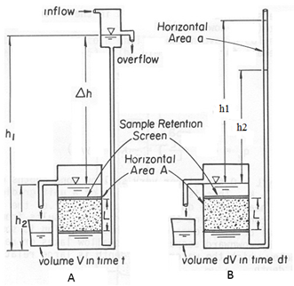
Fig. 23.4.Experimental set for the determination of saturated hydraulic conductivity in Laboratory. A) Constant head method. B) Falling head method.

(Source:http://biosystems.okstate.edu/darcy/Conductivity/Image523.gif : accessed on May 29, 2013)

 

The hydraulic conductivity, K is determined by the equation                 

           (23.10)

 Where,

          V= flow volume in time t

          A= cross sectional area of sample

          L= length of sample

        Δh  = difference in head (h₁-h₂).

 

23.4.1.2 Falling Head Permeameter

The falling-head test is meant for fine-grained soils. Like the constant-head method, the falling-head test is having the direct application of Darcy's law to a one-dimensional, saturated column of soil with a uniform cross-sectional area. The falling-head method differs from the constant-head method in that the liquid that percolates through the saturated column is kept at an unsteady-state flow regime in which both the head and the discharged volume vary during the test. In the falling-head test method, a cylindrical soil sample of cross-sectional area A and length L is placed between two highly conductive plates. The soil sample column is connected to a standpipe of cross-sectional area a, in which the percolating fluid is introduced into the system. Thus, by measuring the change in head in the standpipe from h₁ to h₂ during a specified interval of time t, the saturated hydraulic conductivity can be determined as follows

 

            (23.11)

 

Example 23.1:

If the elevation of h₁ is 35m and the elevation of h₂ is 0m, what is the hydraulic gradient if the distance from h₁ to h₂ is 5.6 km? (Answer in m/km).

Solution:

Given, h₂-h₁= 35m and L=5.6 km

We know: i= (h₂-h₁)/L

          i= 35/5.6 = 6.25m/km.Ans.

 

 

Example 23.2:

Find the velocity of the water flow between two wells located at a distance of 1000 m and the hydraulic conductivity is 114m/day. Drop in elevation between two well is given as 60 m.

 

Solution:

Given: K=114m/day, h₂-h₁=60m, L=1000m

We know, Hydraulic gradient, i = h₂-h₁/L = 60/1000

= 0.06

We know,

V=KI or

V=K(h₂-h₁/L)

V=114m/day * 0.06

V=6.84 m/day. Ans.

 

Example 23.3

An aquifer is 2045 m wide and 28 m thick. Hydraulic gradient across it is 0.05 and its hydraulic conductivity is145m/day. Calculate the velocity of the groundwater as well as the amount of water that passesthrough the end of the aquifer in a day if the porosity of the aquifer is 32%.

 

Solution:

Given:K=145m/day, i= 0.05, W=2045m, D=28m, Porosity =32%

First we must solve for V. We know,

                   V= Ki =145m/day X 0.05

                     =7.25m/day

 

Now that we know V we can determine the discharge (Q) of water through the end of the aquifer

Q= Area. Velocity = A. V= (2045m x 28m) x 7.25m/day

Q=415,135 m³/day.

 

This means that each day, if the aquifer had a porosity of 100%, like a river, would have discharge of 415,135 m³/day.

 

However, the aquifer has porosity of 32 % and hence discharge through aquifer would be

415,135 m3/day X0.32 = 132843.2 m³/day. Ans

 

Example 23.4:

A constant head permeability test was performed on a medium dense sand sample of diameter 60 mm and height 150 mm. The water was allowed to flow under a head of 600 mm. The permeability of sand was 4 x 10^-1 mm/s. Determine (a) the discharge (mm³/s), (b) the discharge velocity.

 

Solution:

(a) We know,

Discharge

(b) Discharge velocity    1.60 mm/s

Example 23.5:

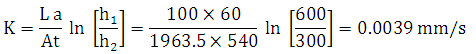
During a falling head permeability test, the head fell from 600 mm to 300 mm in 540 s. the specimen was 50 mm in diameter and had a length of 100 mm. The cross – sectional areaof the stand pipe was 60 mm². Compute the coefficient of permeability of the soil.

 Solution:

Given, a = 60 mm², L= 100 mm, t = 540 s, h₁= 600 mm, h₂= 300 mm.

 

We know,

References

Hansen, V. E., Israelson, O. A., Stinggham, G. (1979). Irrigation Principles and Practice.John Wiley & sons, Inc., New York.

Michael, A.M. (2008). Irrigation Theory and Practice. Vikas Publishing House Pvt Ltd. New Delhi.

Murty, V.V.N. (2002).Land and Water Management Engineering (FourthEdition).Kalyani Publisher, New Delhi.

 

Internet Reference

http://www.angrau.ac.in/media/7380/agro201.pdf

http://gilley.tamu.edu/BAEN464/Handout%20Items/Cuenca%20Book%20Chapter%203%20Soil%20Physics.pdf

http://ilri.org/InfoServ/Webpub/fulldocs/IWMI_IPMSmodules/Module_3.pdf

ftp://ftp.wcc.nrcs.usda.gov/wntsc/waterMgt/irrigation/NEH15/ch1.pdf

 

Suggested Reading

Michael, A.M. (2008). Irrigation Theory and Practice. Vikas Publishing House Pvt Ltd. New Delhi.

http://web.ead.anl.gov/resrad/datacoll/conuct.htm

http://www.fao.org/docrep/r4082e/r4082e03.htm

ftp://ftp.wcc.nrcs.usda.gov/wntsc/waterMgt/irrigation/NEH15/ch1.pdf

http://storm.okstate.edu/bae3313/Lecture/8)%20soilwaterplant%20relationships/soil-water-plant%20relationships.pdf

http://www.angrau.ac.in/media/7380/agro201.pdf