Remote Sensing & GIS Applications 3(2+1)

Lesson 31 Soil Mapping and Soil Erosion Estimation

Traditional soil mapping is conducted with an auger and spade at intervals throughout the landscape. The intervals between inspections can be according to a pre-determined grid (grid-survey) or, more often, are based upon the judgment of the surveyor who uses their knowledge of the inter-relationship between soil type and landscape, geology, vegetation, etc. to determine where to make inspections. Auger borings are supplemented by excavated profile pits at determined points in the landscape. These profile pits are used to demonstrate lateral changes in the soil as well as vertical ones, and are important for the full description of soil type and for the taking of soil samples for chemical, physical and less commonly, biological laboratory analysis. In this way a picture is built up of the soil in a region and its relationship to the landscape in which it lies, (Source: www.soil-net.com/legacy/advanced/soil_mapping.htm).

Soils can be mapped at a range of scales from very detailed at 1:1,250 to 1:5,000 by which the pattern of soils in individual fields can be identified, through to scales of 1:500,000 to 1:500,000,000 which provide only a very generalized picture of the soils of a country or continent. Sometimes soils are mapped with a specific aim in mind, such as the suitability of soils for a particular crop, suitability for irrigation, erosion risk and many other specific needs or environmental threats. Most organized soil surveys in the past have been general purpose surveys. These have the advantage that they provide the basis for many different uses, some of which may yet not be known.

Soil Mapping of Upper DVC Catchment

The Damodar a comparatively small river running a distance of 540 km originates from the Khamarpat at an altitude of 1067m in the district of Jharakhand. It has a drainage area of 24, 235 km². The area shown in Fig 31.1 lies between 23°34' to 24°9' N latitude and 85°00' to 87°00' E Longitude. Mean annual rainfall in the basin is of the order of 1,100 mm and about 80% of rain precipitates during the summer monsoon (June to September). The soil mapping of this study area was done for estimation of soil erosion using USLE. The details of syudy area is available in Mishra (2009).

The soil maps of the study area obtained from AASSLU in the scale of 1:250,000 were traced, scanned and exported to Erdas Imagine 8.5. There were total five maps, four comprised of soils of Bihar (recently renamed as Jharkhand) soils and one map was with soils information of West Bengal soil information. The scanned maps were loaded in ERDAS and georeferenced. Then boundaries of different soil textures were digitized carefully and the polygons representing various soil categories were assigned with different colours for identification. Using ArcView 3.3, digitized soil map was clipped with micro-watershed boundaries and all required data like soil texture, bulk density etc. were extracted for each micro-watershed. The soil is classified mainly on the percentage of available sand into various texture groups such as sandy loam (80.16%), sandy clay loam (9.97%), and loamy sand (9.88%). Fig. 31.1. shows the soil map for Damodar valley catchment. Soil data on texture, structure, permeability and organic matter content by analyzing soil samples were used to derive soil erodibility factor (K).

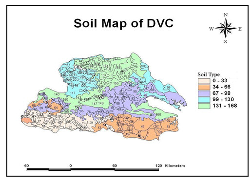
Fig. 31.1. Soil map of DVC. (Source: Shinde, 2009)

31.2 Soil Erosion Estimation and Best Management Practices

31.2.1 Soil Erosion Estimation using USLE

For assessing soil erosion from the watershed, several empirical models based on the geomorphological parameters were developed in the past to quantify the sediment yield. Several other methods such as Sediment Yield Index method and Universal Soil Loss Equation (USLE) are extensively used for prioritization of the watersheds. The USLE formula is given in equation 31.1, has been widely applied at a watershed scale on the basis of lumped approach to catchment scale. The USLE model application in the grid form in GIS environment allows us to analyze soil erosion in much more detail and in more meaningful scene. It is more reasonable to use the USLE on physical basis than to apply it to an entire watershed as a lumped model. Although, GIS permits more effective and accurate application of the USLE model for small watershed, most GIS-model applications are subject to data limitations. The universal soil loss equation (USLE) has widely been used for predicting annual average soil loss for specific areas. In this equation, soil loss (A) is defined as a product of rainfall erosivity factor R, soil erodibility factor K, slope steepness factor S, slope length factor L, cover management factor C, and support practice factor P.

   A= R K L S C P                                                (31.1)

The Soil Conservation Department of DVC, Hazaribagh, Jharakhand (India) has established network of stream gauging stations and sediment observation posts for monitoring hydrological parameters. The time series data on rainfall, runoff, and sediment yield are available through the network of gauging stations. It is possible to analyze the cause-effective relationship between the various factors that affect the hydrologic response of a watershed. Information obtained from such analysis can be used to develop appropriate management plans for soil conservation and water resource development to increase the agricultural productivity of the region on sustainable basis.

31.2.1.1 Development of Model Database for USLE

Rainfall Erosivity (R) Factor

The rainfall erosivity factor (R) map is prepared using daily rainfall data from six stations located in the Upper DVC. The R factor map (Fig. 31.2) is based on 9 year-average rainfall data which is used to calculate annual average R factor values. All the storms do not produce runoff and hence storms more than 12.5 mm were only used in computation.  Eq.31.2, is used for computation of R factor using the daily rainfall amount, (Source: Panigrahi et al., 1996 and Wischmeier, 1959).

R = P²(0.00364log₁₀ P – 0.000062)                     (31.2)

where P= storm depth in mm.

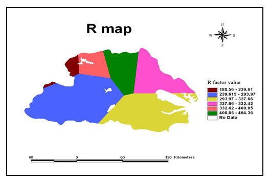
Fig. 31.2. Rainfall erosivity (R) factor map of DVC. (Source: Shinde, 2009)

Soil Erodibility Factor (K)

Soil erodibility factor (K) is a measure of the total effect of a particular combination of soil properties. Some of these properties influence the soil’s capacity to infiltrate rain, and therefore, help to determine the amount of rate of runoff; some influence its capacity to resist detachment by the erosive forces of falling raindrops and flowing water and thereby determine soil content of the runoff. The inter-relation of these variables is highly complex. The K factor in USLE model relates to the rate at which different soils erode. The soil erodibility factor (K) was computed using field and laboratory estimated physico-chemical properties of the surface soils. The laboratory soil analysis was carried out to determine soil texture, structure, permeability and organic matter content for 179 soil samples covering various soil group of the area. The K-factor is computed for each soil type based on the various soil properties using equation 31.3. K factor map generated using GIS is shown in Fig. 31.3, (Source: Wischmeier et al., 1971)

100K = 2.1M^1.14(10^-4) (12 – a) + 3.25 (b –2) + 2.5 (c-3)          (31.3)

Where, K = soil erodibility factor, M = percentage silt, very fine sand and sand > 0.10 mm, a = organic matter content, b = structure of the soil, c = permeability of the soil.

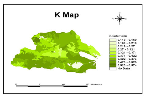
Fig. 31.3. Soil erodibility (K) factor map of DVC. (Source: Shinde, 2009)

Topographic factor (LS)

Topographic factor (LS) is the expected ratio of soil loss per unit area from a field slope to that from a 22.13 m length of uniform 9% slope under otherwise identical conditions. It is this quantity that is significant in rain dependent processes taking place at soil surfaces. Hillslope gradient (S) and length (L) factors are sometimes combined into a topographic factor (LS) while estimating soil erosion. Slope Length factor: The relationship between the slope steepness in percentages (Sp) and slope length in meters (L) was used to generate slope length map. It is given by

L= 0.4 * Sp + 40                                                                                       

By applying this equation the resultant map was prepared for slope length.

Although L and S factors was determined separately, the procedure has been further simplified by combining the L and S factors together and considering the two as a single topographic factor (LS). The combined LS factor layer was generated and shown in Fig. 31.4.

The slope length  modified by Wischmeier and Smith (1965) is used to estimate as  given by-

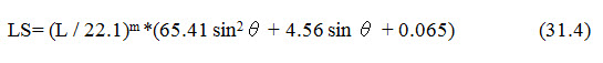
Where, LS is the slope length and gradient factor, θ is angle of the slope and L is slope length in meters and m = 0.5 if the percent slope is 5 or more, 0.4 on slopes of 3.5 to 4.5 percent, 0.3 on slopes of 1 to 3 percent, and 0.2 on uniform gradients of less than 1 percent.

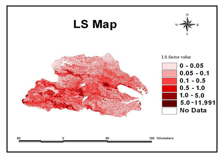
Fig. 31.4. Topographic factor (LS) map of DVC. (Source: Shinde, 2009)

Crop Management Factor (C)

The crop management factor (C) reflects the combined effect of cover, crop sequence, productivity level, length of growing season, tillage practices, residue management and the expected time distribution of erosive rainstorm with respect to seeding and harvesting date in the locality. Actual loss from the cropped field is usually much less than the amount of soil loss for a field kept continuously in fallow conditions. This reduction in soil loss depends on the particular combination of cover, crop sequence and management practices.

Conservation Practice Factor (P)

Presence of soil conservation practices in the region is duly considered in the USLE by including support conservation practice factor (P). Depending upon the LU/LC map, the C factor values are assigned to all classes as shown in Table 31.1. The prepared C factor map is shown in Fig 31.5. In the present study, the land use/land cover map was derived from the supervised classification of LANDSAT ETM images which served as a guiding tool in the allocation of C factor for different land use classes. Conservation practice factor (P) depends on land use/cover information of the study area. If no conservation measures are established, then P factor value of 1 is considered.

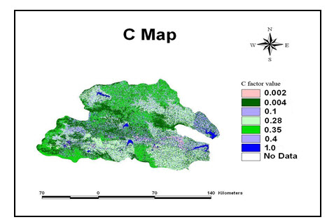
Fig. 31.5. C factor map of DVC. (Source: Shinde, 2009)

Table 31.1. Land use/land cover class and C factor value

Land use/land cover	C value
Forest	0.004
Range	0.1
Water body	1
Urban	0.002
Wetland	0.4
Corn	0.35
Paddy	0.28

(Source: Shinde, 2009)

31.2.1.2 Average Annual Soil Loss using USLE

Annual soil loss based on 9-year average rainfall erosivity factor is termed as average annual soil loss. The annual soil loss for all the micro-watersheds was calculated by using annual average R (based on annual average rainfall data of 1993-2001) and K, LS, C and P factors. The soil erosion rate (t/ha/yr) was estimated as total soil loss of a micro-watershed (t/yr) divided by geographical area of particular micro-watershed (ha). The classification of erosion rate has been given three categories of soil loss. Fig. 31.6 indicates distribution of the micro-watersheds (MWs) of DVC according to soil loss categories. All the layers viz. R, K, LS, C and P were generated in GIS and were overlayed to obtain the product, which gives annual soil loss (A) for the upper DVC. These values gave annual soil loss per hectare per year at pixel level. These values are converted to the loss per pixel in m² (i.e. 84 X 84 m) and all values are added in GIS domain to obtain total annual soil loss per hectare for the upper DVC as a whole. A surface of annual soil loss was overlayed with the micro-watershed map of DVC which contains 705 micro-watersheds to get micro-watershed wise soil loss. All values for each micro-watershed were summed using ‘summarized zone’ option in ArcView GIS 3.3 to obtain soil loss in each micro-watershed. The total loss thus obtained per micro-watershed is then converted to the soil loss/ha/year for the upper Damodar Valley catchment. Micro-watersheds are then classified in different soil loss classes as given in Table 31.2.

Table 31.2. Soil loss categories according to annual average soil loss

Soil loss (t/ha/yr)	Class	Number of Micro-watersheds	Area (km2)
>20	High	345	8503.25
5.0 to 20.0	Medium	159	3981.95
0.0 to 5.0	Low	201	5271.77
Total		705	17756.98

(Source: Shinde, 2009)

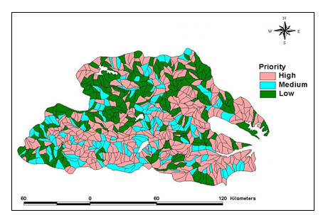
Fig. 31.6. Priority map of DVC Using USLE. (Source: Shinde, 2009)

31.3 Best Management Practices

Adoption of Best Management Practices (BMPs) is required to reduce sediment yield, runoff rate after the deciding of priority of micro-watershed. The various types of BMPs can be suggested to control soil loss for the prioritization soil conservation works in micro-watersheds (Shinde, et al, 2011). BMPs are not exactly same for all micro-watersheds. It varies according to geomorphology of micro-watersheds. The BMPs like afforestation, trenching, bunding, vegetative barriers, sediment basin, bend way weir and different kinds of check dams are selected in different studies. It was found from available treatment data from DVC that, for the completion of treatment in any micro-watershed 3 to 4 years are required. In present study treatment factors (P) were found as 0.7, 0.6 and 0.5 after 1^st, 2^nd and 3^rd year of treatment respectively. While calculating micro-watershed wise soil erosion, P factor applied was 0.5 to those micro-watershed in which treatment has been completed (i.e. after 3^rd year of treatment).

Keywords: Micro-watershed, Soil Mapping, Universal Soil Loss Equation (USLE), Conservation Practice Factor, Best Management Practice Factor.

References

• http://www.soil-net.com/legacy/advanced/soil_mapping.htm

• Misra K., 1999, Watershed Management activities in Damodar Valley Corporation at A Glance, Soil Conservation Department, DVC, Hazaribag, Jharkhand.

• Panigrahi, B., Senapati, P. and Behera, B. (1996). Development of erosion index model from daily rainfall data. Journal of Applied Hydrology, 9 (1 and 2): 17 – 22.

• Shinde V, Sharma A, Tiwari K N and Singh M (2011). Quantitative Determination of Soil Erosion and Prioritization of Micro-Watersheds using Remote Sensing and GIS. Journal of the Indian Society of Remote Sensing, 39(2):181–192.

• Shinde V.T., 2009, Soil Erosion Modeling of Upper Damodar Valley Catchment using GIS, An unpublished M.Tech thesis under the guidance of Prof. K N Tiwari, submitted to Agricultural and Food Engineering Department, IIT Kharagpur.

• Wischmeier, W.H. (1959). A rainfall erosion index for universal soil loss equation. Proceedings of American Soil Science Society, 23: 246-249.

• Wischmeier, W.H., Johnson C.B. and Cross B.V. (1971). A soil erodibility nomograph from farmland and construction sites. Journal of Soil and Water Conservation, 26: 189-193.

• Wishmeier, W.H. and D.D. Smith. 1965. Predicting rainfall erosion losses from cropland east of the Rocky Mountains – Guide for selection of practices for soil and water conservation. USDA Handbook No. 282.

Suggested Reading

• http://www.omafra.gov.on.ca/english/engineer/facts/00-001.htm

• http://www.fao.org/docrep/t1765e/t1765e0e.htm