Reservior & Farm Pond Design 3(2+1)

Lesson 9 Basic Design Concept II

The annual yield of the catchment up to the site of a reservoir, located at the given point along a river, will thus indicate the quantum of water that will annually enter the reservoir, and will thus help in designing the capacity of the reservoir. This will also help to fix the outflows, which are dependent upon the inflows and the reservoir losses.

The amount of water that can be drawn from a reservoir, in any specified time interval, called the reservoir yield, naturally depends upon the inflow into the reservoir and the reservoir losses, consisting of reservoir leakage and reservoir evaporation.

The annual inflow to the reservoir, i.e. the catchment yield, is represented by the mass curve of inflow; whereas, the outflow from the reservoir, called the reservoir yield, is represented by the mass demand line or the mass curve of outflow. Both these curves decide the reservoir capacity, provided the reservoir losses are ignored or separately accounted.

The inflows to the reservoir are however, quite susceptible to variations in land use and land cover changes in the catchment in different years, and may, therefore, vary throughout the prospective life of the reservoir. The past available data of rainfall or runoff in the catchment is, therefore, used to work out the optimum value of the catchment yield. Say, for example, in the past available records of say, 35 years, the minimum yield from the catchment in the worst rainfall year may be as low as say, 100 M.ha-m; whereas the maximum yield in the best rainfall year may be as high as say, 200 M.ha-m. The question then arises, whether the reservoir capacity should correspond to 100 or 200 M.ha-m yield . If the reservoir capacity is provided corresponding to 100 M.ha-m yield, then eventually the reservoir will be filled up every year with a dependability of 100%; but if the capacity is provided corresponding to 200 M.ha-m yield, then eventually the reservoir will be filled up only in the best rainfall year (i.e. once in 35 years) with a dependability of about ×100=3%.

In order to obtain a reasonable agreement, an intermediate dependability percentage value, such as 50 to 75%, may be used to compute the dependable yield or the design yield. The yield, which corresponds to the worst or the most critical year on record, however is called the firm yield or the safe yield. Water available in excess of the firm yield during years of higher inflows, is designated as the secondary yield. Hydropower may be developed from such secondary water. The arithmetic average of the firm yield and the secondary yield is called the average yield.

9.2 Computing Design or Dependable Catchment Yield

The dependable yield, corresponding to a given dependability percentage p, is determined from the past available data of the last 35 years or so. The yearly rainfall data in the reservoir catchment is generally used for this purpose. The rainfall data of the past years is, therefore, used to work out the dependable rainfall value corresponding to the given dependability percentage p. This dependable rainfall value is then converted into the dependable runoff value by using the available empirical formulas connecting the yearly rainfall with the yearly runoff.

It is, however, an adopted practice in Irrigation Departments to plan the reservoir project by computing the dependable yield from the rainfall data, but to start river gauging as soon as the site for the reservoir is decided, and then correlate the rainfall-runoff observations to verify the correctness of the assumed empirical relation between the rainfall and the runoff. Sometimes, on the basis of such observations, the initially assumed yield value may have to be revised. The procedure which is adopted to compute the dependable rainfall value for a given dependability percentage is explained in sub-section 2.3.3 of  Lesson 2.

9.3 Flow Duration Curves for Computing Dependable Flow

Stream flow varies widely over a water year and this variability can be studied by plotting flow duration curves for the given streams. Flow duration curves, also called as discharge frequency curve, is a curve plotted between stream flows(Q) and percent of time the flow is equaled or exceeded (P) (Fig. 9.1, 9.2 and 9.3).

Such a curve can be plotted by first arranging the stream flow values in descending order using class intervals, if the number of individual values is very large. The data to be used can be of daily values, weekly values, or monthly values, If N data values are used, the plotting position of any discharge (or class value) Q is given, as:

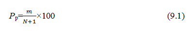
Where, m = order number of that discharge (or class value), and P_P = percentage probability of the flow magnitude being equaled or exceeded.

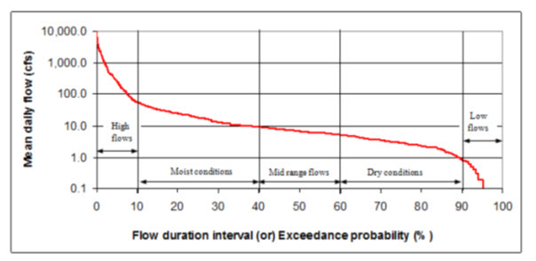
Fig. 9.1.Typical flow duration curve.

(Source:http://www.epa.gov/region6/water/ecopro/watershd/nonpoint/flow-duration-curve-development.pdf)

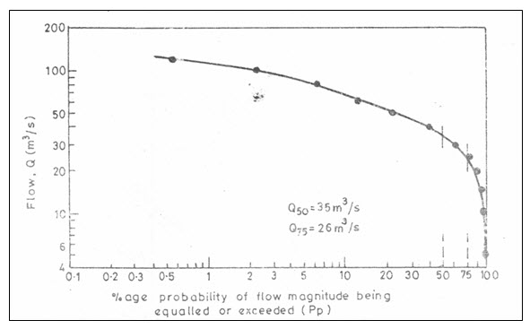
Fig. 9.2. A typical flow duration curve on log-log paper.

(Source: Subramanya, 2009)

The ordinate Q at any percentage probability p(such as 60%), i.e. Q_p, will represent the flow magnitude of the river that will be available for 60% of the year, and is hence termed as 60% dependable flow.Q₁₀₀ for a perennial river can, thus be read out easily from such a curve, Q₁₀₀ for an ephemeral or for an intermittent river shall evidently be zero.

A flow duration curve represents the cumulative frequency distribution, and can be considered to represent the stream flow variation of an average year. Such a curve can be plotted on an ordinary arithmetic scale or semi-log or log-log papers. The following characteristics of flow duration curves have been noticed.

1. The slope of the flow duration curve depends upon the interval of data used. Say for example, a daily stream flow data gives a steeper curve than a curve based on monthly data for the same river. This happens due to smoothening of small peaks in monthly data.

2. The presence of a reservoir on a stream upstream of the gauging point will modify the flow duration curve for the stream, depending upon the reservoir regulation effects on the released discharges.

3. The flow duration curve, when plotted on a log probability paper, is found to be a straight line at least over the central region. From this property various coefficients expressing the variability of the flow in a stream can be developed for the description and comparison of different streams.

4. The flow duration curve plotted on a log-log paper is useful in comparing the flow characteristics of different streams. Say for example, a steep slope on the curve indicates a stream with a highly variable discharges; while a flat slope of the curve indicates a small variability of flow and also a slow response of the catchment to the rainfall. A flat portion on the lower end of the curve indicates considerable base flow. A flat portion on the upper end of the curve is typical of river basins having large flood plains, and also of rivers having large snowfall during a wet season.

5. The chronological sequence of occurrence of the flow gets hidden in a flow duration curve. A discharge of say 500m³/s in a stream will, thus, have a same percentage probability, irrespective of whether it occurred in January or June. This aspect, a serious handicap of such curves, must be kept in mind while interpreting a flow duration curve.        
   

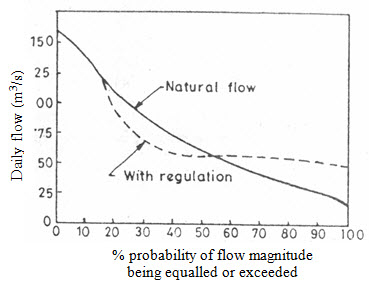
Fig. 9.3. Reservoir regulation effect of F-D curve.

 (Source: Subramanya, 2009)

Flow duration curves find a considerable use in water resources planning and development activities. Some of their important uses are indicated below:

i.   For evaluating dependable flows of various percentages, such as 75%, 60% etc., in the planning of water resources engineering projects.

ii.  In evaluating, the characteristics of the hydropower potential of a river.

iii. In comparing the adjacent catchments with a view to extend the stream flow data.

iv. In computing sediment load and dissolved solids load of a stream.

v.  In the design of drainage systems, and

vi. In flood control studies.

Keywords: Catchment yield, Reservoir capacity, Flow regulation, Dependable flow

References

• Garg, S. K. (2011). Irrigation Engineering and Hydraulic Structures. Khanna Publishers, Twenty fourth Revised Edition. pp. 643-654.

• Subramanya, K. (2009). Engineering Hydrology.Tata McGraw Hill, Third Edition.

Suggested Readings

• http://www.yemenwater.org/wp-content/uploads/2013/03/CATCHMENT-YIELD-ESTIMATION.pdf

• http://www.publish.csiro.au/?act=view_file&file_id=SR9930665.pdf

• http://www.hec.usace.army.mil/publications/TrainingDocuments/TD-3.pdf