Site pages
Current course
Participants
General
Module 1: Formation of Gully and Ravine
Module 2: Hydrological Parameters Related to Soil ...
Module 3: Soil Erosion Processes and Estimation
Module 4: Vegetative and Structural Measures for E...
Keywords
29 March - 4 April
5 April - 11 April
12 April - 18 April
19 April - 25 April
26 April - 2 May
Lesson 16 Unit Hydrograph - II
16.1 Synthetic Unit Hydrograph
To develop unit hydrographs for a catchment, detailed information about the rainfall and the resulting flood hydrograph are needed. However, such information would be available only at a few locations and in a majority of catchments, especially those which are at a remote location; the data would normally be very scanty. In order to construct unit hydrograph for such areas, empirical equations of regional validity which relate the salient hydrograph characteristics to the basin characteristics are available. Unit hydrographs derived from such relationship are known as synthetic unit hydrographs. But these methods being based on empirical correlations are applicable only to the specific regions in which they were developed and should not be considered as general relationship for use in all regions.
Snyder’s Method
Snyder (1938), based on a study of a large number of catchments in the Appalachian Highlands of eastern United States developed a set of empirical equations for synthetic unit hydrograph in those areas. These equations are used in the USA, and with some modifications in many other countries, and constitute what is known as Snyder’s synthetic unit hydrograph (Fig.16.1). This method may be applied in the catchment having area between 25 to 25000 km2 and is based on three parameters namely base width (T), peak discharge (Qp), and lag time (basin lag, tp). The following are the empirical formula involving the three parameters:
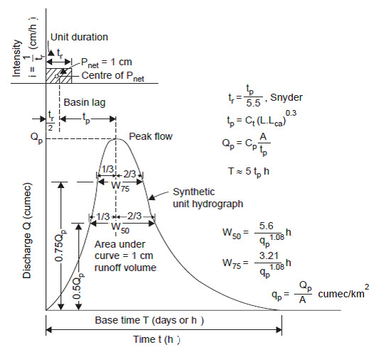
Fig. 16.1. Synthetic unit hydrograph parameters. (Image sources: Raghunath. H.M., 2006)
Lag time, tp = Ct (L Lca)0.3 (16.1)
Standard duration of net rain, tr = tp /5.5 (16.2)
For this standard duration of net rain,
Peak flow, Qp = Cp A/tp (16.3)
Time base in days, T = 3+3(tp/24) (16.4)
Peak flow per km2 of basin, qp = Qp /tp (16.5)
Snyder subsequently proposed an expression to allow for some variation in the basin lag with variation in the net rain duration, i.e., if the actual duration of the storm is not equal to tr given by Eq. (16.2) but is tr/, then
tpr = tp + (tr/ - tr /4) (16.6)
Where,
tpr = basin lag for a storm duration of tr/, and tpr is used instead of tp in Eq. (16.3), (16.4), (16.5).
In the above equations,
tp = lag time (basin lag), h
Ct , Cp = empirical constants (Ct = 0.2 to 2.2, Cp =2 to 6.5, the value depending on the basin characteristics and units)
A = area of the catchment (km2)
L = length of the longest water course, that is of the main stream from the gauging stations (outlet or measuring point) to its upstream boundary limit of the basins, (km) (Fig 16.2)
Lca = length along the main stream from the gauging station (outlet) to a point on the stream opposite the areal center of gravity (centroid) of the basin
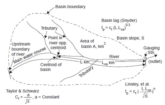
Fig. 16.2. Basin characteristics (Snyder). (Sources: Raghunath, 2006)
As specified by Snyder, the shape of the unit hydrograph is likely to be affected by the basin characteristics like area, topography, shape, slope, drainage density and channel storage. The size and shape of the basin is determined by measuring the length of the main stream channel. The coefficient Ct reflects the size, shape and slope of the basin.
Linsley et al. (1975), gave an expression for the lag time in terms of the basin characteristics as
tp = Ct (LLca/S0.5)n (16.7)
Where, S = basin slope, and the values of n and Ct, when L, Lca were measured in miles are n = 0.38
Ct = 1.2, for mountainous region
= 0.72, for foot hill areas
= 0.35, for valley areas
Taylor and Scwarz found from an analysis (when L and Lca measured in miles) that
Ct = 0.6/S0.5 (16.8)
Time base in h, T = 5(tpr+ tr//2) (16.9)
For developing a synthetic unit hydrograph for a basin for which the stream flow records are not available is to collect the data for the basin like A, L, Lca and to get the coefficients, Ct and Cp from adjacent basins whose streams are gauged and which are hydro meteorologically homogeneous. The three parameters, i.e., the time to peak, the peak flow and the time base are determined from the Snyder’s empirical equations, and the unit hydrograph can be sketched so that the area under the curve is equal to a runoff volume of 1 cm. Empirical formulae have been developed by the US Army Corps of Engineers (1959) for the widths of W50 and W75 of the hydrograph in hours at 50% and 75% height of the peak flow ordinate, respectively, (see Fig. 16.3) as
W50 = 5.6/qp1.08 (16.10)
W75 = W50/1.75 (16.11)
A still better shape of the unit hydrograph can be sketched with these widths (Fig. 16.1). The base time T given by Eq. (16.4) gives a minimum of 3 days even for very small basins and is in much excess of delay attributable to channel storage. In such cases, the author feels T given by Eq. (16.4) be adopted and the unit hydrograph sketched such that the area under the curve gives a runoff volume of 1 cm.
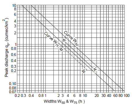
Fig.16.3. Width W50 and W75 for synthetic UG (US Army, 1959). (Sources: Raghunath, 2006)
16.2 Instantaneous Unit Hydrograph
The difficulty of using a unit hydrograph of a known duration has been overcome by the development of the instantaneous unit hydrograph (IUH). The IUH is a hydrograph of runoff resulting from the instantaneous application of 1 cm net rain on the watershed. The IUH in conjunction with the design storm can be used to obtain the design flood by using a convolution integral. The IUH was first proposed by Clark in 1945. The IUH can be developed either directly from the observed data or by adopting conceptual models.
Determination of IUH by S- Curve Hydrograph
In Fig. 16.4, St is the S-curve ordinate at any time t (due to tr-h UG) and S′t is the ordinate at time t of the S-curve lagged by t′r-h, then the t′r-h UGO at time t can be expressed as
U (tr/, t) = (St – St/) tr/tr/ (16.12)
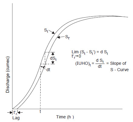
Fig. 16.4. IUH as S-curve derivative. (Sources: Raghunath. H.M., 2006)
As t′r progressively diminishes, i.e., t′r → 0, Eq. (16.12) reduces to the form (as can be seen from Fig. 16.4)
U (0, t) = dSt/dt (16.13)
i.e., the ordinate of the IUH at any time t is simply given by the slope of the S-curve at time t; in other words, the S-curve is an integral curve of the IUH. Since the S-curve derived from the observed rainfall-runoff data cannot be too exact, the IUH derived from the S-curve is only approximate. The IUH reflects all the catchment characteristics such as length, shape, slope, etc., independent of the duration of rainfall, thereby eliminating one variable in hydrograph analysis. Hence, it is useful for theoretical investigations on the rainfall-runoff relationships of drainage basins. The determination of the IUH is analytically more tedious than that of UG but it can be simplified by using electronic computers.
The t′r-UGO can be obtained by dividing the IUH into t′r-hr time intervals, the average of the ordinates at the beginning and end of each interval being plotted at the end of the interval (Fig. 16.5).
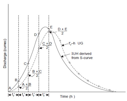
Fig. 16.5. tr/- hr UG derived from IUH. (Sources: Raghunath. H.M., 2006)
Last modified: Monday, 23 September 2013, 5:07 AM