Soil Mechanics

LESSON 20. Flow Net

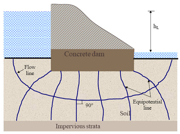
Fig.20.1. Flow net.

From the flow net, the quantity of seepage (Q) is calculated as:

\[Q=k{h_L}{{{N_f}} \over {{N_d}}}\]                      (20.1)

where k is the coefficient of permeability of soil, h_L is head loss from upstream to downstream, N_f is number of flow channels per unit length normal to the plane (in the Figure 20.2, N_f = 2), N_d is the number of equipotential drops (in the Figure 20.2, N_d = 7). If h_L is the total head loss during the flow and N_d is the number of equipotential drops, then Δh = h_L / N_d (as shown in Figure 20.2).

Total head at a point X = h_L - number of drops from upstream × Δh                        (20.2)

Elevation head = -z                                                                                               (20.3)

Pressure head = Total head – Elevation head                                                          (20.4)

It is not necessary to make all the filed elementary squares in a flow net, but a/b ratio (as shown in Figure 20.2) should be same for all the filed elements. If a/b = n, then Eq. (20.1) can be written as:

\[Q=k{h_L}{{{N_f}} \over {{N_d}}}n\]                                                             (20.5)

At the downstream, near the dam (as shown in Figure 20.3), the exit hydraulic gradient (i_exit) can be determined as:

\[{i_{exit}} = {{\Delta h} \over {\Delta L}}\]                                                        (20.6)

If i_exit is greater than the critical hydraulic gradient (i_c), the soil grains at exit get washed away. This phenomenon progresses towards the upstream and forming a free passage of water. This is called Piping in granular soils. The safety factor against piping can be determined as:

\[{F_{piping}}={{{i_c}} \over {{i_{exit}}}}\]                                                       (20.7)

The typical range of F_piping is 5 to 6.

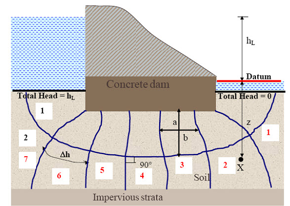
Fig. 20.2. Use of flow net.

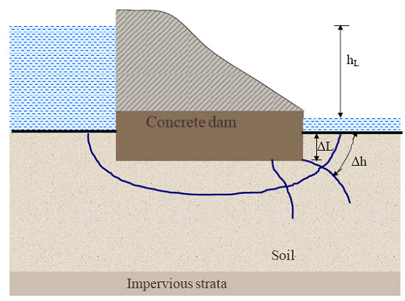
Fig. 20.3 Piping in granular soil.

20.2 Seepage in Anisotropic soil

The Laplace equation presented in previous lesson (lesson 19) is valid for isotropic soil. If soil is anisotropic and coefficient of permeability in x and z direction is not same, the Laplace equation is modified as:

\[{k_x}{{{\partial ^2}h} \over {\partial {x^2}}} + {k_z}{{{\partial ^2}h} \over {\partial {z^2}}}=0\]                               (20.8)

where k_x and k_z are the coefficient of permeability in x and z direction, respectively. The Eq. (20.8) can be written as:

\[\frac{{{\partial ^2}h}}{{\frac{{{k_z}}}{{{k_x}}}\partial{x^2}}}+\frac{{{\partial^2}h}}{{\partial {z^2}}}=0\]            (20.9)

          Convert the x a new coordinate system x' such that

\[x'=x\sqrt {{{{k_z}} \over {{k_x}}}}\]                    (20.10)

and  \[\partial {x'^2}=\partial {x^2}{{{k_z}} \over {{k_x}}}\] , Thus, Eq.(20.9) can be written as:

\[{{{\partial ^2}h} \over {\partial {{x'}^2}}} + {{{\partial ^2}h} \over {\partial {z^2}}}=0\]                (20.11)

The Eq.(20.11) is Laplace equation for isotropic soil w.r.t x' and z coordinates. Here x coordinate is transformed to x' coordinate [as per Eq. (20.10)] for converting anisotropic soil medium into a fictitious isotropic medium (by keeping z coordinate unchanged). Thus, during the coordinate transformation horizontal dimension (x dimension) is multiplied by \[\sqrt {{{{k_z}} \over {{k_x}}}}\]  . The value of coefficient of permeability for transformed section is taken as:

\[k'=\sqrt {{k_x}{k_z}}\]                  (20.12)

Thus, in this case the quantity of seepage (Q) is calculated as:

\[Q=\sqrt {{k_x}{k_z}} {h_L}{{{N_f}} \over {{N_d}}}\]               (20.13)

20.3 Seepage in Non-Homogeneous Section

Figure 20.4 shows the Change in direction of flow lines at intersection of two soil layers with different permeability. In such situation, the condition is:

\[{{{k_1}} \over {{k_2}}}={{\tan {\alpha _1}} \over {\tan {\alpha _2}}}\]            (20.14)

If k₁ > k₂, the flow lines get defected towards the normal after the intersection (i.e. a₁ > a₂). Similarly, If k₁ < k₂, the flow lines get defected away from the normal after the intersection (i.e. a₁ < a₂). If the permeability of one layer is 10 times more than the permeability of other layer, then it is assumed that no resistance for lowing of water is offered from more pervious layer, thus, no deflection correction is necessary.

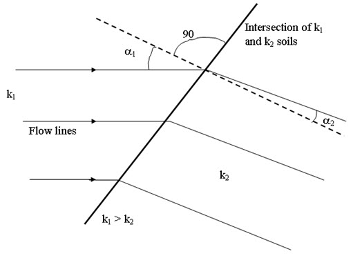
Fig.20.4. Change in direction of flow lines at intersection of two soil layers  

                with different permeability.

 

References

Ranjan, G. and Rao, A.S.R. (2000). Basic and Applied Soil Mechanics. New Age International Publisher, New Delhi, India.

PPT of Professor N. Sivakugan, JCU, Australia.

Suggested Readings

• Ranjan, G. and Rao, A.S.R. (2000) Basic and Applied Soil Mechanics. New Age International Publisher, New Delhi, India.

• Arora, K.R. (2003) Soil Mechanics and Foundation Engineering. Standard Publishers Distributors, New Delhi, India.

• Murthy V.N.S (1996) A Text Book of Soil Mechanics and Foundation Engineering, UBS Publishers’ Distributors Ltd. New Delhi, India.

• PPT of Professor N. Sivakugan, JCU, Australia (www.geoengineer.org/files/permy-Sivakugan.pps‎).