Site pages
Current course
Participants
General
MODULE 1. Fundamentals of Soil Mechanics
MODULE 2. Stress and Strength
MODULE 3. Compaction, Seepage and Consolidation of...
MODULE 4. Earth pressure, Slope Stability and Soil...
Keywords
29 March - 4 April
5 April - 11 April
12 April - 18 April
19 April - 25 April
26 April - 2 May
LESSON 23. Consolidation Test
23.1 Introduction
In the laboratory, the consolidation of a saturated soil specimen is conducted in a device called oedometer as shown in Figure 23.1. The test is done for undisturbed soil sample collected from field. The test is done by applying incremental external loading as shown in Figure 23.2. After allowing full consolidation, the next increment of loading is applied [as shown in Figure 23.2 (a)]. The change in void ratio (Δe1) due to application of loading increment, Δq1 can be determined as:
\[\Delta {e_1} = {{\Delta {H_1}} \over H}(1 + {e_0})\] (23.1)
where H is the initial thickness of the soil sample, ΔH1 is the change in thickness or height (compression) of the sample due to the application of Δq1, e0 is the initial void ratio of the sample. After completing the loading test, unloading test is also conducted as shown in Figure 23.2(b). In case of loading, as the stress increases void ratio decreases and for unloading case, as the stress decreases void ratio increases. After determining the void ratio (e) due to application of incremental pressure (p), e – log σv' is plotted (as shown in Figure 23.3) for both loading and unloading conditions. The σ'v is the effective vertical stress which is determined from the applied incremental loading. The slope of the straight portion of the loading curve is compression index (Cc) and slope of the unloading curve is swelling index. Thus, the Compression index can be determined as: Cc = (e1 – e2) / (log σ'2 – log σ'1). According to Skempton (1944): Cc = 0.009 (wL – 10), where wL is the liquid limit.
The coefficient of compressible (av) can be determined as:
\[{a_v}={{\Delta e} \over {\Delta {{\sigma '}_v}}}\] (23.2)
where Δe is the change in void ratio due to the change in effective vertical stress Δσ'v. Similarly, the coefficient of volume change or coefficient of volume compressibility (mv) can be determined as:
\[{m_v}={{{a_v}} \over {1 + {e_0}}} = {{\Delta e} \over {\Delta {{\sigma '}_v}}}\left( {{1 \over {1 + {e_0}}}} \right)\] (23.3)
where e0 is the initial void ratio of the soil sample.

Fig. 23.1. Laboratory consolidation test.
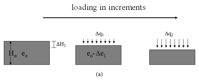
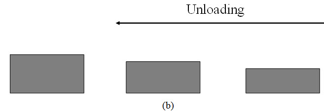
Fig. 23.2. Loading arrangement (a) Loading (b) Unloading.

Fig. 23.3. e – log σv' plot.
23.2 Over Consolidation Ratio
Casagrande (1936) proposed to determine the pre-consolidation stress from e – log σv' plot as shown in Figure 23.4. Locate the point O where there is smallest radius of curvature. Draw a line OA parallel to stress or x axis. Draw a tangent OB at point O. Draw the line OC such that it bisects the angle AOB. Extend the straight portion of the e – log σv' plot. The stress corresponding to the point of intersection of extended line and OC line is the pre-consolidation pressure the soil was subjected. If the present effective overburden pressure σ'v0 is equal to the preconsolidated pressure σc' (maximum past effective overburden pressure), the soil is normally consolidated soil. However, if σ'v0 < σc', the soil is overconsolidated. Thus, overconsolidation ratio (OCR) is defined as: OCR = σc'/σ'v0.
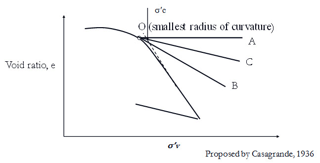
Fig. 23.4. Determination of preconsolidation stress .
23.3 Settlement Calculation
Figure 23.5 shows the e – log σv' plots for normally consolidated and overconsolidated clay for settlement calculation. For normally consolidated clay the settlement (S) can be determined as:
\[S={{{C_c}} \over {1 + {e_0}}}H{\log _{10}}\left( {{{{{\sigma '}_{v0}} + \Delta {{\sigma '}_v}} \over {{{\sigma '}_{v0}}}}} \right)\] (23.4)
where H is total thickness of the soil layer.
For over-consolidated clay: Case 1: σ'v0+Δσ'v < σ'c
\[S={{{C_s}} \over {1 + {e_0}}}H{\log _{10}}\left( {{{{{\sigma '}_{v0}} + \Delta {{\sigma '}_v}} \over {{{\sigma '}_{v0}}}}} \right)\] (23.5)
Case 2: σ'v0 < σ'c < σ'v0+Δσ'v
\[S={{{C_s}} \over {1 + {e_0}}}H{\log _{10}}\left( {{{{{\sigma '}_c}} \over {{{\sigma '}_{v0}}}}} \right)\] + \[{{{C_c}} \over {1 + {e_0}}}H{\log _{10}}\left( {{{{{\sigma '}_{v0}} + \Delta {{\sigma '}_v}} \over {{{\sigma '}_c}}}} \right)\] (23.6)
where Cs is the swelling index.
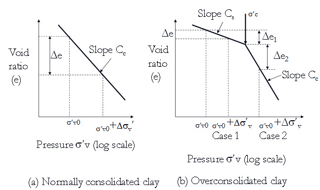
Fig. 23.5. Settlement calculation (a) Normally consolidated clay
(b) Overconsolidated clay .
References
Ranjan, G. and Rao, A.S.R. (2000). Basic and Applied Soil Mechanics. New Age International Publisher, New Delhi, India.
PPT of Professor N. Sivakugan, JCU, Australia.
Suggested Readings
Ranjan, G. and Rao, A.S.R. (2000) Basic and Applied Soil Mechanics. New Age International Publisher, New Delhi, India.
Arora, K.R. (2003) Soil Mechanics and Foundation Engineering. Standard Publishers Distributors, New Delhi, India.
Murthy V.N.S (1996) A Text Book of Soil Mechanics and Foundation Engineering, UBS Publishers’ Distributors Ltd. New Delhi, India.
PPT of Professor N. Sivakugan, JCU, Australia (www.geoengineer.org/files/consol-Sivakugan.pps).
Last modified: Tuesday, 24 September 2013, 10:15 AM