Machine Design 3(2+1)

LESSON 4. DESIGN FOR COMBINED LOADING & THEORIES OF FAILURE

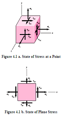
If the stress vectors acting on three mutually perpendicular planes passing through the point are known, stress vector acting on any other arbitrary plane at that point can be determined. Let us consider three mutually perpendicular planes (x-plane, y-plane and z-plane) passing through a point as shown in figure 4.1a. Normal and shear stress components acting on these planes are:

Plane	Normal Stress Component	Shear Stress Components
x-plane	sx	τxy, τxz
y-plane	sy	τyx, τyz
z-plane	sz	τzx, τzy

 

 

 

 

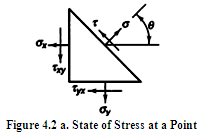
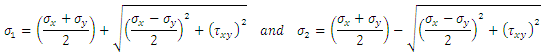
For equilibrium, in most cases, cross shears are equal i.e. τ_xy = τ_yx, τ_yz = τ_zy and τ_xz =τ_zx. Therefore, six components of stress are required to completely define thestate of stress. State of stress, when the stresses on one surface are zero, is called plane stress. Figure 4.1b shows the state of plane stress, with normal and shear stress components on the z-plane to be zero (s_z = τ_zx = τ_zy =0). Stress acting on any oblique plane, whose normal makes an angle \[\theta \] with the x-axis, for state of plane stress, can be determined with the help of figure 4.2a. Considering equilibrium of forces, normal (σ) and shear stress (\[\tau \]) components acting on this arbitrary oblique plane are given by,

From strength consideration, it is important to find the plane of maximum normal stress and plane of maximum shear stress and their magnitudes.  Differentiating the expression for normal stress (s) with respect to q and equating it to zero, we get:

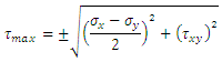
This gives two values of \[\theta \] i.e. two planes, which are perpendicular to each other. One has maximum value of normal stress and the other has minimum value. These two planes are called principal planes as the shear stress component along these planes is zero. Normal stress components on these planes are called Principal Stresses and are given by,

Differentiating the expression for shear stress (\[\tau \]) with respect to q and equating it to zero, we get

This also gives two values of \[\theta \] i.e. two mutually perpendicular planes, which make an angle of 45° with the principal planes. Shear stress component along these planes, also called principal shear stress is given by,

 

State of stress at any point or maximum principal stresses and maximum principal shear stress at any point can be determined from the abov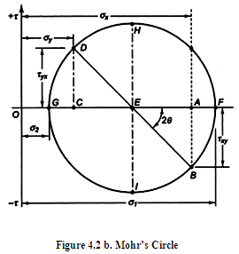e relations or graphically with the help of Mohr’s Circle as shown in figure 4.2b. Normal stresses are plotted along abscissa and shear stresses are plotted along the ordinate. Tensile normal and clockwise shear stresses are considered to be positive and compressive normal and anticlockwise shear stresses are considered to be negative. Mohr’s Circle can be constructed and used to find maximum principal stresses and maximum principal shear stress as given below:

1. Draw OA = σ_x, OC = σ_y, AB = \[\tau \]_xy and CD = \[\tau \]_yx.

2. Join BD to get point E, intersection of AC and BD.

3. Construct Mohr’s Circle with E as centre and BD as diameter.

4. OF gives maximum principal stress σ₁ and OG represents minimum principal stress σ₂.

5. EH and EI give the maximum principal shear stress ±_{\[\tau \]max}.

4.2 Theories of Failure

In the previous article, it has been discussed that how the state of stress can be determined for any point in a component subjected to combined loads and how to get the value of maximum principal stresses and maximum principal shear stress developed in the component. Now for designing components subjected to combined load, it is important to relate this complex state of stress to the properties of material (yield strength, ultimate tensile strength, percentage elongation etc.), which are obtained from the simple tension test, so that the failure in such conditions can be predicted. This relationship is provided by ‘Theories of Elastic Failure’, which are discussed below.

4.2.1 Maximum Principal Stress Theory

This theory is credited to W.A. J. Rankine. It states that failure of any mechanical component subjected to complex state of stress occurs whenever

one of the three principal stresses equals or exceeds the strength i.e. whenever maximum tensile stress exceeds the uniaxial tensile strength or maximum compressive stress exceeds the uniaxial compressive strength. If σ₁,σ₂ and σ₃ are the three principal stresses with 

σ₁ ≥ σ_2 ≥  σ₃ , theory says that to avoid failure,

Therefore, design equations based on maximum principal stress theory can be written as:

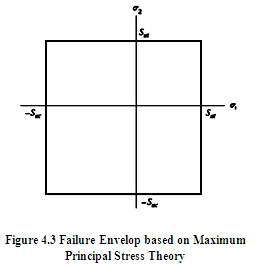
Figure 4.3 shows the failure envelop based on maximum principal stress theory, for plane stress case (σ₂  = 0) . Area is bounded by lines  \[{\sigma _1} = {S_{ut}},{\sigma _1} =  - {S_{uc}},{\sigma _2} = {S_{ut}}and{\sigma _2} =  - {S_{uc}}\]. Test data shows that this theory is suitable for predicting failure of brittle materials and is not recommended for ductile materials.

4.2.2 Maximum Shear Stress Theory

This theory is credited to C.A. Coulumb, H Tresca and J.J. Guest.  It states that any mechanical component subjected to any combination of loads will fail whenever maximum shear stress exceeds shear strength of the material (i.e. shear stress at the time of yielding in the standard specimen of tension test). Figure 4.4 shows Mohr’s Circle for 3-dimensional stress with σ₁,σ₂ and σ₃ as principal stresses such that σ₁ ≥ σ₂ ≥ σ₃. Three principal shear stresses are then given by,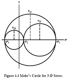

As evident from the figure 4.4, maximum shear stress \[{\tau _{max}} = {\tau _{13}} = \left( {{\sigma _1} - {\sigma _3}} \right)/2\] .

Now, for simple tension test,σ₁ = σ_x & σ₂ = σ₃ = 0, giving . Also yielding in simple tension test starts when σ₁ = S_yt. Therefore, maximum shear stress at the time of yielding in simple tension test is \[{\tau _{max}}\] = S_yt / 2. Thus, design equation based on maximum shear stress theory can be written as:

Note that for plane stress case, σ₃ = 0 and.  

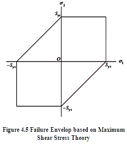
Graphical representation of maximum shear stress theory, giving failure envelop for state of plane stress (σ₃=0), is shown in Figure 4.5. According to this theory, for state of plane stress, yielding starts when σ₁ - σ₂ = S_yt . But in 1^st and 3^rd quadrant of this (σ₁ - σ₂) plot, σ₁ and σ₂ are of same nature with (σ₁ - σ₂) > σ₂ and yielding may start when  reaches the yield strength,S_yt . Therefore, in 1^st and 3^rd quadrant, area is bounded by lines σ₁ = ±S_yt and σ₂ = ±S_yt. Whereas in 2^nd and 4^th quadrant, area is bounded by lines, which represent the condition where maximum shear stress reaches the shear strength of the material i.e. \[{\tau _{max}}\] = S_sy = S_yt /2 . This theory is suitable for predicting failure of ductile materials but is a little conservative.

4.2.3 Maximum Distortion Energy Theory

This theory is credited to M.T. Hueber, R. von-Mises and H. Hencky. It states that a mechanical component subjected to combined loads fails when the distortion strain energy per unit volume at any point in the component reaches or exceeds the distortion strain energy per unit volume of standard specimen of simple tension test, at the time of yielding.

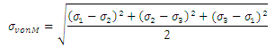
This theory gives a value of equivalent stress, called von-Mises Stress, which is defined as the value of uniaxial tensile stress that would produce the same level of distortion energy as the actual stress involved. It is given by,

To avoid failure of the component, this von-Mises stress should not exceed yield strength of the material. Therefore design equation based on maximum distortion energy theory can be written as,

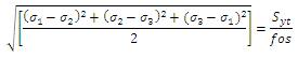
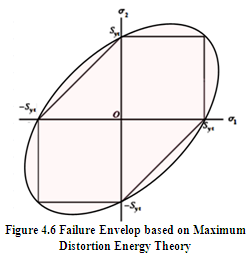
Figure 4.6 shows the failure envelop, based on maximum distortion energy theory, for state of plane stress. Experimental results have proved that this theory is the best suitable for predicting failure of ductile materials. It can be proved that according to maximum distortion energy theory, yield strength in shear is 0.577 times yield strength in tension i.e. S_ys = 0.577 S_yt.

 

 

References

1. Design of Machine Elements by VB Bhandari

2. Mechanical Engineering Design by J.E. Shigley

3. Analysis and Design of Machine Elements by V.K. Jadon

4. Advanced Mechanics of Solids by L.S. Srinath

5. Fundamentals of Machine Component Design by R.C. Juvinall & K.M. Marshek

6. Machine Elements in Mechanical Design by Robert L. Mott