Machine Design 3(2+1)

LESSON 7. DESIGN FOR DYNAMIC LOADING - II

7.1.1 Design for Infinite Life

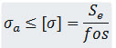
If the stress developed in a component is kept below the endurance limit, it can survive for infinite number of cycles or can have infinite life. Thus endurance limit is the design criteria in this case and the design equation can be written as:

7.1.2 Design for Finite Life

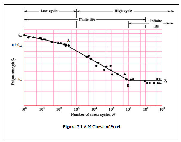
When components are designed to survive for 10³ to 10⁶ number of cycles, it is called design for finite life. For S-N curve of steel shown in figure 7.1, line AB represents this region.

To design for finite life, fatigue strength is taken as design criteria. Fatigue strength for required number of stress cycles can be determined graphically from the S-N curve or mathematically by using the equation of line AB. Or alternatively, for a known value of induced stress, number of cycles that the component will survive can be calculated. S-N curve is a log-log plot and co-ordinates of points A and B are:

\[A(3,lo{g_{10}}\left( {0.9{S_{ut}}} \right)andB\left( {6,lo{g_{10}}{S_e}} \right)\]

Ordinate of point A is approximately 90% of the ultimate tensile strength.

Equation of line AB can be written as,

\[lo{g_{10}}\left( {{S_f}} \right) = blo{g_{10}}N + c\]  or \[{S_f} = {N^b}{10^c}\]

Where, b and c are constants that can be determined using co-ordinates of A and B.

\[b = \frac{1}{3}lo{g_{10}}\left( {\frac{{{S_e}}}{{0.9{S_{ut}}}}} \right)andc = lo{g_{10}}\left( {\frac{{{{(0.9{S_{ut}})}^2}}}{{{S_e}}}} \right)\]

7.2 Design for Fluctuating Stresses

In this case, mean value of stress has a non-zero value and both static and variable components of stress contribute to the failure. Figure 7.2 shows the scatter of failure points obtained from various experiments performed with different combinations of σ_m and σ_a. Observing these results, Soderberg, Goodman and Gerber have proposed three different theories, defining the boundary line between the safe and unsafe region on the σ_m vs σ_a plot. Soderberg line, Goodman Line and Gerber Parabola are described in table 7.1 and are shown in figure 7.2. When stress amplitude (_σa) is zero, stress is purely static and S_yt or S_ut are the criteria of failure. These are plotted on the abscissa, along which s_m is plotted. When the mean stress (σ_m) is zero, stress is completely reversing and S_e is the criteria of failure. It is plotted on the ordinate, along which σ_a is plotted.

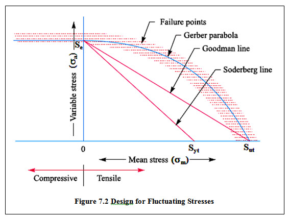Table 7.1 Design for Fluctuating Stresses

Criteria	Soderberg Line	Goodman Line	Gerber Parbola
Description	Line joining Se on the ordinate to Syt on the abscissa.	Line joining Se on the ordinate to Sut on the abscissa.	Parabolic curve joining Se on the ordinate to Sut on the abscissa.
Equations	\[\frac{{{\sigma _m}}}{{{S_{yt}}}} + \frac{{{\sigma _a}}}{{{S_e}}} = 1\]	\[\frac{{{\sigma _m}}}{{{S_{ut}}}} + \frac{{{\sigma _a}}}{{{S_e}}} = 1\]	\[{\left( {\frac{{{\sigma _m}}}{{{S_{ut}}}}} \right)^2} + \frac{{{\sigma _a}}}{{{S_e}}} = 1\]
Considering Factor of Safety	\[\frac{{{\sigma _m}}}{{{S_{yt}}/fos}} + \frac{{{\sigma _a}}}{{{S_e}/fos}} = 1\]	\[\frac{{{\sigma _m}}}{{{S_{ut}}/fos}} + \frac{{{\sigma _a}}}{{{S_e}/fos}} = 1\]	\[{\left( {\frac{{{\sigma _m}}}{{{S_{ut}}/fos}}} \right)^2} + \frac{{{\sigma _a}}}{{{S_e}/fos}} = 1\]
Final Design Equation	\[\frac{{{\sigma _m}}}{{{S_{yt}}}} + \frac{{{\sigma _a}}}{{{S_e}}} = \frac{1}{{fos}}\]	\[\frac{{{\sigma _m}}}{{{S_{ut}}}} + \frac{{{\sigma _a}}}{{{S_e}}} = \frac{1}{{fos}}\]	\[{\left( {\frac{{{\sigma _m}}}{{{S_{ut}}}}} \right)^2}.fos + \frac{{{\sigma _a}}}{{{S_e}}} = \frac{1}{{fos}}\]

 

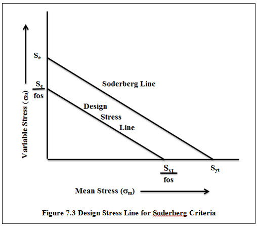
As discussed in the case of static loading, allowable stress or design stress is obtained by dividing S_ut or S_yt by factor safety. Similarly, in the present case, taking factor of safety reduces the safe region as shown in figure 7.3 for Soderberg line.

 

References

1. Mechanical Engineering Design by J.E. Shigley

2. Analysis and Design of Machine Elements by V.K. Jadon

3. Design of Machine Elements by VB Bhandari

4. Design of Machine Elements by M. F. Spotts

5. Design of Machine Elements by C.S. Sharma & K. Purohit

6. Machine Elements in Mechanical Design by Robert L. Mott