Site pages
Current course
Participants
General
Module 1_Fundamentals of GW
Module 2_Well Hydraulics
Module 3_Design, Installation and Maintenance of W...
Module 4_Groundwater Assessment and Management
Module 5_Principle, Design and Operation of Pumps
Module 6_Performance Characteristics, Selection an...
Keywords
Lesson 9 General Procedure for Analyzing Groundwater Flow Towards Wells
9.1 Introduction
Analytical solutions of the equations governing groundwater flow for a particular combination of the characteristics of the aquifer and the well can be obtained on the basis of suitable assumptions concerning type of flow and aquifer properties. The aquifer properties include transmissivity, storage coefficient, nature of the boundaries of the flow domain, homogeneity and isotropy as well as the depth and areal extent of the aquifer. Despite the simplifying assumptions inherent in the analytical solutions, they provide pragmatic answers to the groundwater problems if applied judiciously.
When a production well tapping an aquifer of infinite areal extent is pumped at a constant rate, the radius of influence of the well expands radially from the pumping well. In practice, flow towards a pumping well is mostly unsteady (transient). A number of specific situations of unsteady flow towards groundwater wells are discussed in Sarma (2009). For each flow situation, the governing equation, appropriate boundary conditions and initial condition are defined, and then solutions to the governing flow equations are presented. Note that for deriving analytical solutions, several simplfying assumptions are made, of which the basic assumptions required to be made for analyzing either steady or unsteady groundwater flow to wells are described in the subsequent section.
In this lesson, a general procedure for the analysis of groundwater flow to wells is demonstrated, which has been adapted from Sarma (2009). The analysis of steady groundwater flow to wells is discussed in Lesson 10 and that of transient groundwater flow to wells is discussed in Lesson 11.
9.2 Basic Assumptions for Analyzing Groundwater Flow to Wells
The following are the basic assumptions made for analyzing steady or transient groundwater flow to wells:
(1) The aquifer is bounded on the bottom by a confining layer.
(2) The groundwater level of the aquifer is horizontal and not changing with time prior to the start of pumping.
(3) All changes in the position of the groundwater level are due to the effect of the pumping well alone.
(4) All geologic formations are horizontal and of infinite horizontal extent.
(5) The aquifer is homogeneous and isotropic.
(6) All flow is radial towards the well.
(7) Groundwater flow is horizontal.
(8) Darcy’s law is valid.
(9) The pumping well and the observation wells are fully penetrating.
(10) The pumping well has an infinitesimal diameter (i.e., negligible storage) and is 100% efficient (i.e., no well losses).
(11) Groundwater has a constant density and viscosity.
9.3 General Procedure
A critical examination of the procedures adopted in different cases for analyzing groundwater flow to wells reveals that there exists certain commonality in the procedures. For example, for the cases of transient groundwater flow to wells, by taking Laplace transform of the governing partial differential equation (p.d.e.) and the associated boundary and initial conditions, the equation can be reduced to the p.d.e. in terms of space coordinates only. Further, in the case of groundwater flow towards partially penetrating wells, two of the boundaries of the flow region are parallel to each other. Such problems can be simplified by using Finite Fourier transforms and thereby reducing the p.d.e. to a Bessel differential equation in one space variable (Sarma, 2009). The associated initial and boundary conditions are also transformed accordingly. Thereafter, the Bessel differential equation in the transformed domain subject to the corresponding transformed boundary conditions can be solved. By taking inverse transforms, first the inverse Finite Fourier transforms and then the inverse Laplace transform for transient flow cases, the solution to the original problem can be obtained. Thus, for solving the governing p.d.e. for most cases of groundwater flow to wells, a general procedure can be adopted. Various steps involved in the general procedure are as foolows (Sarma, 2009):
Step 1: If the groundwater flow equation describes transient flow condition, take Laplace transform for the governing p.d.e. as well as the associated initial and boundary conditions.
Step 2: If the resulting p.d.e. involves parallel boundaries, take an appropriate Finite Fourier transform for the p.d.e. and the boundary conditions obtained in Step 1. Note that if the parallel boundaries constitute barrier boundaries (impermeable or no-flow boundaries), the Finite Fourier cosine transform is to be used. However, for the case of parallel boundaries constituting recharge boundaries, the Finite Fourier sine transform is to be used.
Step 3: The resulting Bessel differential equation of zero order is solved using the standard solution procedure and the properties of Bessel functions. It is worth mentioning that the differential equation obtained for all the cases is the modified Bessel differential equation of order zero for which standard solutions are available in the literature.
Step 4: The solution of the Bessel differential equation, subject to the associated boundary conditions, which are also transformed through Finite Fourier transforms, is then inverse transformed using the appropriate inverse Fourier transform (sine or cosine as the case may be).
Step 5: The resulting expression of the solution for the drawdown is transformed by using the inverse Laplace transform to obtain the solution of the original p.d.e.
The above procedure, which involves only five steps, can be applied to many cases of groundwater flow to wells. This generic procedure is demonstrated in this lesson using two examples of transient groundwater flow to wells in a leaky confined aquifer.
9.4 Illustrative Examples
9.4.1 Example 1: Transient Groundwater Flow to a Partially Penetrating Well in Leaky Confined Aquifers
Occurrence of leakage flow from or into the aquifer being pumped is a function of the potential difference between the aquifer and the aquifer on the other side of the aquitard through which leakage takes place. Thus, in the case of leaky aquifers, while there is a scope for recharge to the aquifer being pumped, the flow continues to be transient unless the rate of recharge is equal to the rate of pumping.
Considering radial symmetry of flow towards wells and the basic assumptions mentioned in Section 9.2, except for the assumption ‘the pumping well is fully penetrating’ and referring to Fig. 9.1, the governing p.d.e. for the case of transient flow of groundwater towards a partially penetrating pumping well in a homogeneous and isotropic leaky confined aquifer of infinite aerial extent can be written as:
 (9.1)
(9.1)
Euation (9.1) is subject to the following initial and boundary conditions:
Initial Condition (I.C.): ![]()
Boundary Conditions (B.C.): ![]()
and 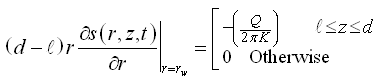 (9.2)
(9.2)
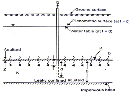
Fig. 9.1. Transient flow towards a partially penetrating well in a leaky confined aquifer. (Source: Sarma, 2009)
Where, s = drawdown in the leaky confined aquifer, r = radial distance from the pumping well, Q = constant pumping rate, rw = radius of the pumping well, B = leakge factor, T = transmissivity of the leaky confined aquifer, S = storage coefficient of the leaky confined aquifer, b = thickness of the leaky confined aquifer, K = hydraulic conductivity of the leaky confined aquifer, K’ = hydraulic conductivity of the aquitard (leaky confining layer), b’ = thickness of the aquitard, and the meaning of other symbols are as illustrated in Fig. 9.1.
Step 1: Since the p.d.e. [Eqn. (9.1)] describes transient flow, applying the first step of taking Laplace transform of the p.d.e. and the associated initial and boundary conditions [Eqn. (9.2)] leads to:
 (9.3)
(9.3)
Subject to transformed initial condition and boundary conditions given as:
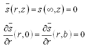
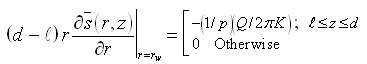 (9.4)
(9.4)
Step 2: Equation (9.3) is a p.d.e. in two space dimensions. Further the flow is such that the flow domain (Fig. 9.1) has two parallel no-flow boundaries (at z = 0, and z = b). Hence, taking the Finite Fourier cosine transform for the p.d.e. [Eqn. (9.3)] and the associated boundary conditions [Eqn. (9.4)] leads to:
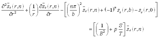
Or,
 (9.5)
(9.5)
In which, 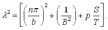 .
.
Equation (9.5) is subject to:
![]()
and 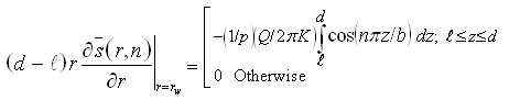 (9.6)
(9.6)
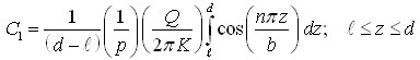
Step 3: Equation (9.5) is a modified Bessel differential equation of order zero, for which the general solution is given as:
![]()
The value of the constants C1 and C2 can be evaluated using Eqn. (9.6) and the properties of the modified Bessel functions K0 and I0. Thus, C2 = 0 and
Therefore,
 (9.7)
(9.7)
Step 4: Taking inverse finite cosine Fourier transform of Eqn. (9.7) leads to:
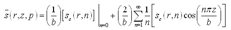
The first term on the R.H.S. (with n = 0) is equal to:
In which, 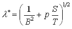 (9.8)
(9.8)
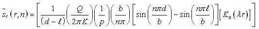
and the second term on the R.H.S. is equal to:
Therefore,
 (9.9)
(9.9)
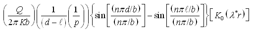
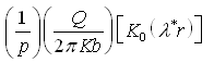
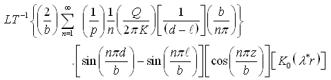
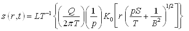
Step 5: Taking inverse Laplace transform of Eqn. (9.9), the first term becomes:
![]()
 (A)
(A)
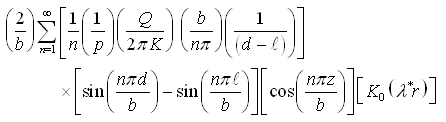
and
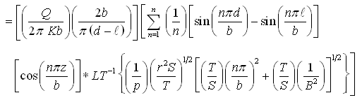
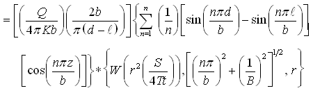 (B)
(B)
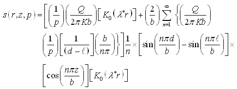
Hence, s(r,z,t) = (A) + (B)
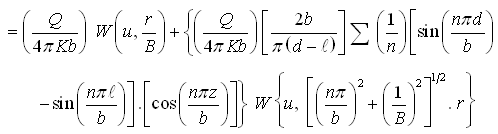
(9.10)
Thus, in this example, due to the nature of the groundwater flow condition, all the five steps were used to obtain the expression for drawdown around the pumping well. However, in many cases, all the five steps many not be required. Nevertheless, by following the sequence and using the relevant steps, the corresponding solution can be obtained. One such case is presented below as Example 2.
9.4.2 Example 2: Transient Flow to a Fully Penetrating Well in Leaky Confined Aquifers
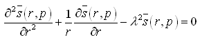
The partial differential equation governing transient flow towards a pumping well fully penetrating a homogeneous and isotropic leaky confined aquifer of infinite aerial extent (Fig. 9.2) written in the radial coordinate system in terms of drawdown (s) is given as:
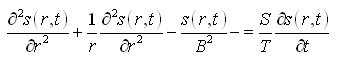 (9.11)
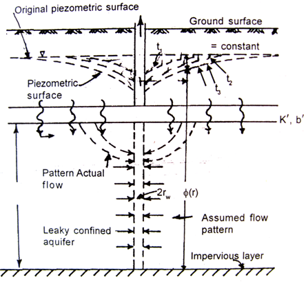
Fig. 9.2. Transient flow towards a fully penetrating well in a leaky confined aquifer. (Source: Sarma, 2009)
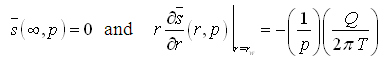
Equation (9.11) is subject to the following initial and boundary conditions:
Initial condition: s (r, 0) = 0
Boundary conditions: s (¥, t) = 0
and 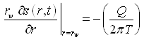
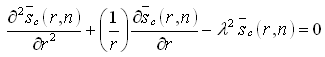
Step 1: Taking Laplace transformation of the p.d.e. and the associated initial and boundary conditions leads to:
 (9.12)
Subject to:
 (9.13)
Where, 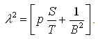
Step 2: This step is not required in this case because the p.d.e. is a function of s and r only.
Step 3: Equation (9.12) is a modified Bessel differential equation of zero order and of first kind, the solution of which is familiar.
Step 4: Evaluation of Eqn. (9.12) in terms of the boundary conditions leads to:
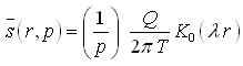 (9.14)
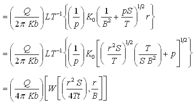
Step 5: Taking the inverse Laplace transform of Eqn. (9.14) leads to the solution of the original problem as follows:
Or, 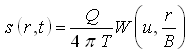 (9.15)
Where, 
Equation (9.15) is known as Hantush-Jacob formula, which is described in Lesson 11. This equation is limited to the conditions that the leakage derived from the storage of the aquitard is negligible and the r/B ratio is small, preferably less than 0.1. It can be seen that Eqn. (9.15) reduces readily to the solution of the case of non-leaky confined aquifer (i.e., Theis equation), if B is set to a very large value (¥).
Note thatt in this example, only four steps are required to obtain the solution. For the further details on the derivation of analytical solutions to various types of well hydraulics problems, interested readers are referred to Sarma (2009) and Batu (1998).
References
Batu, V. (1998). Aquifer Hydraulics: A Comprehensive Guide to Hydrogeologic Data Analysis. John Wiley & Sons, New York.
Sarma, P.B.S. (2009). Groundwater Development and Management. Allied Publishers Pvt. Ltd., New Delhi.
Suggested Readings
Sarma, P.B.S. (2009). Groundwater Development and Management. Allied Publishers Pvt. Ltd., New Delhi.
Batu, V. (1998). Aquifer Hydraulics: A Comprehensive Guide to Hydrogeologic Data Analysis. John Wiley & Sons, New York.
Raghunath, H.M. (2007). Ground Water. New Age International (P) Limited, New Delhi.
Todd, D.K. (1980). Groundwater Hydrology. John Wiley & Sons, New York.
Last modified: Friday, 7 February 2014, 11:53 AM