Ground Water,Wells and Pumps 3(2+1)

Lesson 11 Unsteady Groundwater Flow to Wells

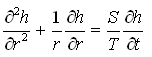                                               (11.1) 

Where, h = hydraulic head, r = radial distance from the pumping well, S = storage coefficient of the aquifer, T = transmissivity of the aquifer, and t = time. 

For steady groundwater flow to pumping wells in a homogeneous and isotropic confined aquifer system, Eqn. (11.1) reduces to the Laplace equation in the polar coordinate system: 

                                           (11.2)    

 

Moreover, for transient axisymmetric groundwater flow to pumping wells in a homogeneous and isotropic leaky confined aquifer system, Eqn. (5.49) of Lesson 5 can be expressed in the polar coordinate form as: 

                                      (11.3) 

For steady axisymmetric groundwater flow to pumping wells in a homogeneous and isotropic leaky confined aquifer system, Eqn. (11.3) reduces to: 

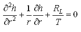                                             (11.4) 

Where, R_L is the leakage rate, which can be determined by the Darcy’s law as: 

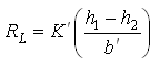                                                (11.5) 

Where, h₁ = hydraulic head at the top of the aquitard (leaky confining layer), h₂ = hydraulic head in the aquifer just below the aquitard, K¢ = vertical hydraulic conductivity of the aquitard, and b¢ = thickness of the aquitard. 

Solutions of the above transient radial flow equations for a variety of boundary conditions have yielded a number of useful equations. These solutions have been obtained by using Laplace transforms, finite Fourier transforms, Bessel functions, and error functions (e.g., Sarma, 2009; Batu, 1998). These solutions can be used to calculate transient drawdown in a pumping well and/or nearby observation wells or discharge of the pumping well, if the aquifer parameters and the remaining variables are known. Conversely, if aquifer parameters are unknown, pumping test (described in Lesson 13) can be conducted and the observed time-drawdown data or time-recovery data can be analyzed to determine hydraulic parameters of different aquifer systems.

 

11.2 Solution of Unsteady Flow to Wells in Confined Aquifers

11.2.1 Theis Equation

Theis (1935) was the pioneer in solving Eqn. (11.1) and obtained an analytical solution for the transient flow of groundwater to pumping wells tapping a confined aquifer (Fig. 11.1). For solving Eqn. (11.1), Theis made the following assumptions in addition to the basic assumptions mentioned in Lesson 10:

       (1)       The aquifer is confined (i.e., it is bounded on the top and bottom by confining layers).

       (2)       Groundwater flow to the pumping well is under unsteady-state condition.

       (3)       There is no source of recharge to the aquifer. That is, all the pumped water comes from the aquifer storage.

       (4)       The aquifer is compressible and the water is released instantaneously from the aquifer storage with the decline in head due to pumping.

       (5)       The well is pumped at a constant rate.

 

The analytical solution was found by Theis based on the analogy between groundwater flow and heat conduction in solids and considering following initial condition and two boundary conditions: 

 

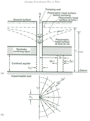
Fig. 11.1. Unsteady flow to a fully penetrating well in a confined aquifer: (a) Vertical cross section; (b) Plan. (Source: Batu, 1998)

 

Initial condition: h(r,0) = h₀ for all r (i.e., the hydraulic head before pumping at any distance r from the pumping well is equal to the initial hydraulic head).

Boundary conditions: (i)  for all t (t >0). That is, the hydraulic head at an infinite radial distance for all time is constant at h_o (initial hydraulic head).

(ii) 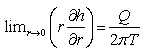 (i.e., the rate of groundwater withdrawal is constant at the pumping well).

 

Given the above initial and boundary conditions, the ultimate solution is expressed as follows: 

                                         (11.6) 

The dimensionless variable u appearing in Eqn. (11.6) is defined as: 

                                                   (11.7) 

Where, h = hydraulic head at distance r from the pumping well, h_o = hydraulic head just before the start of pumping (t = 0), Q = constant pumping rate, s(r,t) = h_o−h = drawdown at a distance r from the pumping well at time t, S = storage coefficient of the aquifer, T = transmissivity of the aquifer, and t = time since pumping started.

 The exponential integral , is known as well function for confined aquifers or Theis well function and is generally denoted by W(u). Thus, Eqn. (11.6) can also be written as follows: 

                                                     (11.8) 

Eqn. (11.6) or (11.8) is called Theis equation or Non-equilibrium equation. As W(u) is a complicated function, its calculation is not straightforward. Therefore, the values of W(u) for different values of u have been presented in a tabular form, which can be found in standard books on groundwater hydrology or hydrogeology. 

 

11.2.2 Cooper-Jacob Equation

H. H. Cooper and C. E. Jacob in 1946 suggested a simple but approximate method to compute Theis well function [W(u)] by replacing W(u) with an infinite series as follows: 

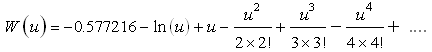       (11.9) 

Cooper and Jacob (1946) observed that after the pumping well is running for some time, the value of u becomes small and the higher-power terms (involving u², u³, u⁴ and so on) of Eqn. (11.9) become so small that they can be easily ignored. Thus, Cooper and Jacob (1946) assumed that when the values of u are small (u ≤ 0.01), only first two terms of Eqn. (11.9) are sufficient to compute W(u). With this assumption, Eqn. (11.6) or Eqn. (11.8) can be written as:    

 

                             (11.10)

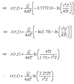      (11.11a)

 

Or, 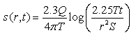                                    (11.11b)

 

Eqn. (11.11a) or (11.11b) is well known as Cooper-Jacob equation. Note that the Cooper-Jacob equation does not require the table of Theis well function, and hence it can be evaluated directly by using a calculator. However, the limitation of this equation is that it is valid only when u ≤ 0.01. For u ≤ 0.01, the error is less than 1% which can be considered negligible for practical purposes. Therefore, while using the Cooper-Jacob equation, it is necessary to check whether its use is justified for solving a given problem.     

The Theis equation and the Cooper-Jacob equation can be used for forward calculation (i.e., to calculate transient drawdown in a pumping well and/or observation wells or discharge of the pumping well or distance of the drawdown observation point or radius of influence) if the aquifer parameters and the remaining variables are known. In addition, they can also be used for calculating aquifer parameters (T and S), which involves the analysis of time-drawdown data or time-recovery data (observed during pumping tests) following standard procedures as described in Lesson 14.

 

11.3 Solution of Unsteady Flow to Wells in Leaky Confined Aquifers

As we know that in leaky confined aquifers, leakage takes place through the confining layers from an adjacent aquifer (Fig. 11.2). Therefore, when leaky confined aquifers are pumped, the water withdrawn from leaky confined aquifers comes from aquifer storage as well as from leakage. Pumping gradually increase the leakage rate due to increase in head difference between the leaky confined aquifer and the adjacent aquifer. The net effect of this leakage is to reduce the drawdown in the confined aquifer compared to that expected from an ideal confined aquifer (Theis-type response). The solutions of unsteady flow to wells in leaky confined aquifers have been obtained for two situations. In the first situation, leakage is considered as the flow across a confining layer (aquitard) without storage in the confining layer. In the second situation, however, it is considered that the storage in the aquitard is also a source of leakage. These two types of solutions are discussed below.

 

11.3.1 Hantush-Jacob Equation (Without Storage in the Aquitard)

Hantush and Jacob (1955) derived an analytical solution for the transient flow of groundwater to pumping wells tapping a leaky confined aquifer system (Fig. 11.2). In this case, they considered that all the water flowing to the pumping well comes from either elastic storage in the confined aquifer and/or leakage across the confining layer (aquitard). No water is derived from elastic storage in the aquitard. For solving Eqn. (11.3), Hantush and Jacob (1955) made the following assumptions besides the basic assumptions mentioned in Lesson 10:

       (1)       Groundwater flow to the pumping well is under unsteady-state condition.

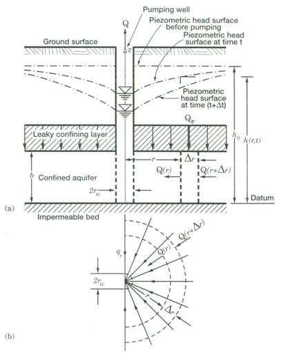
Fig. 11.2. Unsteady flow to a fully penetrating well in a leaky confined aquifer: (a) Vertical cross section; (b) Plan. (Source: Batu, 1998)

 

       (2)       The confined aquifer is leaky and the leakage occurs into the aquifer through the confining layer (aquitard) from an adjacent aquifer wherein hydraulic head remains constant during pumping.

       (3)       Storage in the confining layer (aquitard) is negligible. That is, no water is released from storage in the aquitard when the aquifer is pumped.

       (4)       The confining layer that overlies or underlies the leaky confined aquifer has a uniform hydraulic conductivity (K¢) and thickness (b¢).

       (5)       Groundwater flow is vertical in the confining layer and radial in the leaky confined aquifer.

       (6)       The leaky confined aquifer is compressible and the water is released instantaneously from the aquifer storage with the decline in head due to pumping.

       (7)       The well is pumped at a constant rate.

 

Given the above assumptions and considering appropriate initial and boundary conditions, Hantush and Jacob (1955) found an analytical solution to Eqn. (11.3) which is known as Hantush-Jacob equation and it is given as: 

                                   (11.12) 

Where, is called well function for leaky confined aquifers or Hantush well function, and is expressed as: 

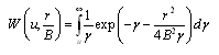                                                                  (11.13) 

, and B = leakage factor which is expressed as: 

                                                   (11.14) 

Since W(u,r/B) is a much more complicated function than the Theis well function mentioned above, its calculation is complex. Therefore, the values of W(u,r/B) have been presented in a tabular form for different values of u and r/B by Hantush (1956), which can also be found in standard books on groundwater hydrology or hydrogeology.  

Like the Theis equation, the Hantush-Jacob equation can also be used for forward calculation as well as for the calculation of aquifer parameters (T, S, and B) from pumping-test data of leaky confined aquifers without storage in the aquitard. Moreover, the rate that water is being withdrawn from elastic storage in the confined aquifer (q_s) at a given time (t) since pumping started can be estimated from the following equation (Fetter, 1994):   

                                       (11.15) 

If the total discharge (rate of groundwater withdrawal) at time t is Q and the water withdrawn from aquifer storage at that time is q_s, then the rate of leakage through the aquitard at that time (q_L) can be estimated as: 

                                 (11.16) 

If the well is pumped long enough, all the water will be coming from leakage across the confining layer and no water will be coming from elastic storage in the confined aquifer. This situation creates steady-state flow condition in the leaky confined aquifer and it occurs when . In this case, the steady drawdown in the leaky confined aquifer is given as follows (Hantush and Jacob, 1955): 

                                        (11.17) 

Where, K₀ = Zero-order modified Bessel function of the second kind. The values of K₀(x) are available in Hantush (1956), and are also tabulated in standard books on groundwater hydrology or hydrogeology. Like the Thiem equation, Eqn. (11.17) can be used for forward calculation as well as for the calculation of aquifer parameters.    

 

11.3.2 Hantush Equation (With Storage in the Aquitard)

If the assumption ‘no water is released from storage in the aquitard when the aquifer is pumped’ made in the previous case is not valid, then the solution for leaky confined aquifers with a contribution of water from storage in the aquitard must be used (Hantush, 1960). This solution is based on the basic assumptions mentioned in Lesson 10 as well as all of the assumptions used in the previous section (Section 11.3.1), except the assumption that storage in the aquitard is negligible. Thus, in this case, it was considered that some water comes from elastic storage in the aquitard. This case has two solutions as described below. 

Solution 1:  During the early part of pumping when   (where b’, S’ and K’ are the thickness, storage coefficient and hydraulic conductivity of the aquitard, respectively), all the water will come from elastic storage in the aquifer and the aquitard. In this case, the analytical solution to the governing equation [Eqn. (11.3)] was derived by Hantush (1960) as follows: 

                                        (11.18)      

Where, H(u,β) is called modified well function for leaky confined aquifers or modified Hantush well function, and β is expressed as: 

                                             (11.19) 

The remaining symbols in Eqn. (11.18) have the same meaning as defined earlier. Eqn. (11.18) is known as Hantush equation.  The values of H(u,β) have been presented in a tabular form for different values of u and β by Hantush (1961), which can also be found in standard books on groundwater hydrology or hydrogeology. The Hantush equation can also be used for forward calculation as well as for the calculation of aquifer parameters from pumping-test data of leaky confined aquifers with storage in the aquitard.

 

Solution 2: If sufficient time elapses, the aquifer will reach equilibrium and all of the water will be coming from drainage from the overlying aquifer (source bed). The time to reach this equilibrium is given as: 

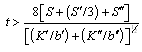                                 (11.20) 

Where, K” and b” are the hydraulic conductivity and saturated thickness of the overlying aquifer (source bed), respectively.

If the value of r_w/B is less than 0.01, then the solution is: 

                                           (11.21) 

This is the same solution as that for steady-state (equilibrium) flow condition in the case where no water comes from elastic storage in the aquitard [i.e., Eqn. (11.17)]. This is so because all the water comes from the source bed (overlying aquifer).                           

 

11.4 Solution of Unsteady Flow to Wells in Unconfined Aquifers

11.4.1 Neuman Equation for Unconfined Aquifers with Delayed Yield

Unlike confined aquifer, unconfined aquifers essentially yield water by two mechanisms when they are pumped: (i) like the confined aquifers, the decline in water pressure (hydraulic head) in the unconfined aquifer yields water due to elastic storage of the aquifer which is characterized as S_s (specific storage of the aquifer); and (ii) the declining water table also yields water as it drains (dewaters) under gravity from the aquifer material, which is characterized as S_y (specific yield of the aquifer). The second mechanism of water yielding dominates in most unconfined aquifers. However, the gravity drainage (dewatering) of pores is a slow process, and hence it does not keep pace with the rapid decline of the water table during pumping.  Large-size pores drain faster than the small-size pores. As a result, some water drains from above the cone of depression (which was saturated before pumping) much later than the fall of the water table and this vertical (or gravity) drainage continues for some time (Fig. 11.3b). This typical response of unconfined aquifers to pumping is termed ‘delayed yield’ or ‘delayed gravity response’ (Boulton, 1954; Neuman, 1972), which is briefly explained below.

 

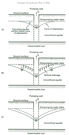
Fig. 11.3. Development of cone of depression in an unconfined aquifer: (a) Initial cone of depression; (b) Gravity drainage of the initial cone of depression; (c) Cone of depression under equilibrium condition.

(Source: Batu, 1998)

 

Fig. 11.4. Illustration of delayed gravity response and its effect on drawdown in unconfined aquifers. (Source: Batu, 1998)

 

There are three distinct phases (time segments) of time-drawdown curves in the unconfined aquifer showing delayed yield (Fig. 11.4):

1. First Segment (Early Segment): In this segment, which lasts for some seconds to a few minutes of pumping, water is released essentially instantaneously from aquifer storage by the aquifer compaction and by water expansion similar to confined conditions. Almost all water supplied to the well comes from the aquifer storage in the saturated zone. Gravity water above the hydraulic head within the cone of depression still has not reached the saturated zone (Fig. 11.3a). The storage coefficient during this phase is close to a confined aquifer of the same porous material as that of the unconfined aquifer and is denoted as S (Fig. 11.4).

(2) Second Segment (Intermediate Segment): This segment displays a gradual flattening in the time-drawdown slope caused by gravity-drainage replenishment from the pore spaces above the cone of depression, which were saturated before pumping. It indicates that the gravity water is reaching the saturated zone (Fig. 11.3b), but is still not in equilibrium with the saturated flow. The flat (straight-line) portion of the time-drawdown curve (Fig. 11.4) indicates that the rate of gravity drainage is equal to the rate of pumping from the aquifer.

(3) Third Segment (Late Segment):  This segment represents equilibrium between the gravity drainage and the saturated flow when the delayed gravity response ceases (Fig. 11.3c). Such an equilibrium condition is achieved when the rate of gravity drainage is equal to the rate of decline in the water table. This hydraulic condition occurs in an unconfined aquifer after several minutes to several days of pumping. The storage properties during this phase are those of a truly unconfined aquifer and are termed ‘specific yield’ (S_y) (Fig. 11.4).

 

The flow of groundwater towards a pumping well in unconfined aquifers showing delayed yield is described by the following partial differential equation (Neuman and Witherspoon, 1969):

                                 (11.22) 

Where, K_r = radial hydraulic conductivity of the unconfined aquifer, K_v = vertical hydraulic conductivity of the unconfined aquifer, S_s = specific storage of the unconfined aquifer, z = elevation above the base of the aquifer, and the remaining symbols have the same meaning as defined earlier.

 

Neuman (1975) solved Eqn. (11.22) after making some specific assumptions in addition to the basic assumptions mentioned in Lesson 10. The solution is known as Neuman equation, which is given as follows: 

                                (11.23) 

Where, W(u_a, u_y, h) is known as well function for unconfined aquifers or Neuman well function, and the dimensionless parameters u_a, u_y and h are defined as:

 

 (applicable for early drawdown data)                          (11.24)

 

 (applicable for later drawdown data)                         (11.25)

 

                                                                                    (11.26)

 

Where, S = storativity or storage coefficient of the unconfined aquifer, T = transmissivity of the unconfined aquifer, h₀ = initial saturated thickness of the unconfined aquifer, K_h = horizontal hydraulic conductivity of the unconfined aquifer, and the remaining symbols have the same meaning as defined earlier. The values of W(u_a, u_y, h) have been presented in a tabular form by Neuman (1975), which can also be found in standard books on groundwater hydrology or hydrogeology.  Like the Theis equation, the Neuman equation can also be used for forward calculation as well as for the calculation of aquifer parameters (K_h, K_v, S and S_y) from pumping-test data obtained from the unconfined aquifer exhibiting delayed yield.

 

11.4.2 Theis Equation for Unconfined Aquifers without Delayed Yield

The Theis equation for confined aquifers can also be applied to unconfined aquifers provided that the basic assumptions are satisfied. In general, if the drawdown is small in relation to the saturated thickness of the unconfined aquifer, reasonably good approximations are possible (Stallman, 1965). Furthermore, it has been found that many unconfined aquifers do not exhibit delayed yield, i.e., the time-drawdown curve does not show three distinct phases as discussed above. In this case also, the Theis equation can be used for unconfined aquifers without much error. Alternatively, a refined approach as suggested in Section 10.2.5 of Lesson 10 for the application of the Thiem equation to unconfined aquifers can be followed while using the Theis equation for unconfined aquifers. This approach has proved to be very effective for solving the flow problems related to unconfined aquifers.   

 

11.5 Solution of Unsteady Flow to Cavity Wells

The solutions for unsteady drawdown behavior around a pumped cavity well (Fig. 11.5) have been obtained by Kanwar and Chauhan (1974) and Chauhan et al. (1975). These solutions are based on the following assumptions:

(1)    The confined aquifer is homogeneous, isotropic and has an infinite areal extent and an extensive thickness.

(2)    A spherical sink of infinitesimal radius r in the form of a non-penetrating well with sides impermeable and hemispherical bottom is situated at the boundary of the impermeable layer and the confined aquifer.

(3)    The water removed from aquifer storage is discharged instantaneously with decline in head.

(4)    The water is pumped at a constant rate and the specific storage coefficient is constant.

 

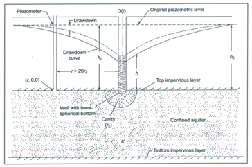
Fig. 11.5. Illustration of unsteady spherical flow into a cavity well in a confined aquifer. (Source: Michael et al., 2008)

 

The following partial differential equation (Michael et al. (2008) governs the unsteady (transient) spherical flow in a homogeneous and isotropic non-leaky confined aquifer (Fig. 11.5): 

                                          (11.27) 

Where, h = hydraulic head in the confined aquifer, r = radial distance from the centre of the cavity well, S_s = specific storage of the confined aquifer, K = hydraulic conductivity of the confined aquifer, and t = time since pumping started.

 

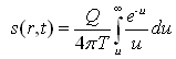
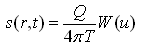
Chauhan et al. (1975) obtained the solution of Eqn. (11.27) for drawdown at a distance r from the pumping well (cavity well) at any time t as follows: 

                                   (11.28) 

Where, s(r,t) = drawdown at a distance r and time t, Q = constant discharge from the cavity well, K = hydraulic conductivity of the confined aquifer, and u is defined as: 

                                                (11.29) 

Like the Theis equation, Eqn. (11.28) can also be used for forward calculation as well as for the calculation of aquifer parameters (K, S_s and S) from pumping-test data obtained using a cavity well. The procedure for determining hydraulic properties of confined aquifers using cavity wells can be found in Michael et al. (2008).

 

References

Batu, V. (1998). Aquifer Hydraulics: A Comprehensive Guide to Hydrogeologic Data Analysis. John Wiley & Sons, New York.

Boulton, N.S. (1954). The drawdown of the water table under nonsteady conditions near a pumped well in an unconfined formation. Proc. Inst. Civil Engrs., 3: 564-579.

Chauhan, H.S., Jaiswal, C.S. and Seth, H.B.S. (1975). Analysis of flow to non-penetrating well in an artesian aquifer. Institution of Engineers (India) Journal-Civil, 56: 45-47.

Cooper, H.H. and Jacob, C.E. (1946). A generalized graphical method for evaluating formation constants and summarizing well field history. Transactions, American Geophysical Union, 27: 526-534.

Fetter, C.W. (1994). Applied Hydrogeology. Third Edition, Prentice Hall, NJ.

Hantush, M.S. (1956). Analysis of data from pumping tests in leaky aquifers. Transactions, American Geophysical Union, 37: 702-714.

Hantush, M.S. (1960). Modification of the theory of leaky aquifers. Journal of Geophysical Research, 65: 3713-3725.

Hantush, M.S. (1961). Tables of the function   New Mexico Institute of Mining and Technology Professional Paper 103, 12 pp.

Hantush, M.S. and Jacob, C.E. (1955). Nonsteady radial flow in an infinite leaky aquifer. Transactions, American Geophysical Union, 36: 95-100.

Kanwar, R.S. and Chauhan, H.S. (1974). Unsteady spherical flow to a non-penetrating well in an artesian aquifer. Journal of Agricultural Engineering, ISAE, 11: 14-21.

Michael, A.M., Khepar, S.D. and Sondhi, S.K. (2008). Water Well and Pump Engineering. Second Edition, Tata McGraw Hill Education Pvt. Ltd., New Delhi.

Neuman, S.P. (1972). Theory of flow in unconfined aquifers considering delayed response of the water table. Water Resources Research, 8: 1031-1045.

Neuman, S.P. (1975). Analysis of pumping test data from anisotropic unconfined aquifers considering delayed gravity response. Water Resources Research, 11: 329-342.

Neuman, S.P. and Witherspoon, P.A. (1969). Applicability of current theories of flow in leaky aquifers. Water Resources Research, 5: 817-829.

Sarma, P.B.S. (2009). Groundwater Development and Management. Allied Publishers Pvt. Ltd., New Delhi.

Stallman, R.W. (1965). Effects of water table conditions on water level changes near pumping wells. Water Resources Research, 1: 295-312.

Theis, C.V. (1935). The relation between the lowering of the piezometric surface and rate and duration of discharge of a well using groundwater storage. Transactions, American Geophysical Union, 16: 519-524.

 

Suggested Readings

Todd, D.K. (1980). Groundwater Hydrology. John Wiley & Sons, New York.

Fetter, C.W. (2000). Applied Hydrogeology. Fourth Edition. Prentice Hall, NJ.

Sarma, P.B.S. (2009). Groundwater Development and Management. Allied Publishers Pvt. Ltd., New Delhi.

Raghunath, H.M. (2007). Ground Water. New Age International (P) Limited, New Delhi.

Schwartz, F.W. and Zhang, H. (2003). Fundamentals of Ground Water. John Wiley & Sons, New York.