Ground Water,Wells and Pumps 3(2+1)

Lesson 14 Analysis of Pumping-Test Data

As discussed in Lesson 12, there are several methods for the determination of hydraulic parameters of aquifer systems. However, the pumping test (or ‘aquifer test’) is the standard and most widely used method for determining the hydraulic parameters of aquifers, viz., transmissivity (T), hydraulic conductivity (K), storage coefficient (S), specific yield (S_y) and leakage factor (B). As mentioned in Lesson 13, the pumping test yields aquifer parameters averaged over a large and representative volume of the aquifer, and hence it is more reliable than the methods providing essentially point estimates (e.g., slug/bail tests and laboratory methods). Different types of pumping tests are available which provide varying types of pumping-test data for confined, unconfined and leaky aquifer systems. Depending on the type of pumping-test data and the type of aquifer in which the test is conducted, a wide range of methods are available for analyzing pumping-test data in order to determine aquifer parameters. Table 14.1 summarizes commonly used methods for analyzing pumping-test data obtained from confined, unconfined and leaky confined aquifers. The detailed discussion on each of the methods is beyond the scope of this course, and hence only selected methods are discussed in this lesson. Interested readers may refer to Kruseman and de Ridder (1994), Fetter (1994), Batu (1998), Kasenow (2001), Schwartz and Zhang (2003), and Michael et al. (2008) for further details about the methods described in this lesson, together with the discussion on other methods of pumping-test data analysis.

 

In the past, the analyses of pumping-test (aquifer-test) data for determining aquifer parameters or for determining hydraulic characteristics of production wells were done manually only, which is cumbersome and somewhat subjective. However, with a rapid advancement in the computer technology and numerical techniques, it is possible to perform such analyses using a PC (laptop or desktop). Commercial software packages such as AquiferTest developed by the Waterloo Hydrogeologic, Inc., Canada (http://www.swstechnology.com), AQTESOLV (http://www.aqtesolv.com/) and Aquifer^win32 (http://www.aquifer-test.com/), among some others, are available which enable us to analyze different types of pumping-test data easily and efficiently in considerably less time. These software packages are based on either graphical approaches or numerical approaches to aquifer-test data analysis. In addition, the developer of this course, Prof. Madan Kumar Jha, has copyrighted a user-friendly software package named GA-AquiAnalyzer which facilitates the analysis of aquifer-test data by the genetic algorithm (GA) technique (Samuel and Jha, 2003)      

 

Table 14.1. Commonly used methods for pumping-test data analysis

Sl. No.	Type of Aquifer	Type of Pumping-Test Data	Name of Methods
1	Confined Aquifer	(i) Time-Drawdown data	Theis Type Curve Method Cooper-Jacob Straight-Line Method
		(ii) Unsteady Distance-Drawdown data	Cooper-Jacob Straight-Line Method
		(iii) Quasi-Steady/Steady Distance-Drawdown data	Thiem Method Graphical Method
		(iv) Recovery data: -    Time-Residual Drawdown data -    Time-Recovery data	Residual Drawdown-Time Ratio Method Cooper-Jacob Straight-Line Method
2	Unconfined Aquifer without Delayed Yield	(i) Time-Drawdown data	Theis Type Curve Method Cooper-Jacob Straight-Line Method
		(ii) Unsteady Distance-Drawdown data	Cooper-Jacob Straight-Line Method
		(iii) Quasi-Steady/Steady Distance-Drawdown data	Thiem Method Graphical Method
		(iv) Recovery data: -    Time-Residual Drawdown data -   Time-Recovery data	Residual Drawdown-Time Ratio Method Cooper-Jacob Straight-Line Method
3	Unconfined Aquifer with Delayed Yield	(i) Time-Drawdown data	Type-Curve Method Neuman Straight-Line Method
		(ii) Quasi-Steady/Steady Distance-Drawdown data	Thiem Method Graphical Method
4	Leaky Confined Aquifer without Storage in Aquitards	(i) Time-Drawdown data	Walton Type-Curve Method Hantush Inflection-Point  Method
		(ii) Quasi-Steady/Steady Distance-Drawdown data	Type-Curve Method
5	Leaky Confined Aquifer with Storage in Aquitards	(i) Time-Drawdown data	Hantush Type-Curve Method
		(ii) Quasi-Steady/Steady Distance-Drawdown data	Type-Curve Method

 

14.2 Determination of Confined Aquifer Parameters

As shown in Table 14.1, the hydraulic parameters of confined aquifer systems can be determined using time-drawdown data, distance-drawdown data and recovery data. The methods used for analyzing these pumping-test data are discussed in this section. 

 

14.2.1 Theis Type-Curve Method

It is a graphical method for analyzing time-drawdown data. In this method, the field-data curve is matched with the standard curve known as Theis type curve (Fig. 14.1) and then the hydraulic parameters of confined aquifers viz., T and S can be determined using the Theis equation [Eqn. (11.8)] as follows: 

 

Theis equation can be rearranged as:                                          (14.1)

 

Also, can be rearranged as:                                           (14.2)

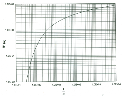
Fig. 14.1. Theis Type Curve for confined aquifers. (Source: Roscoe Moss Company, 1990)

 

The step-by-step procedure for determining confined aquifer parameters from time-drawdown data by the Theis Type-Curve method is as follows:

Step 1: Construct Theis Type Curve by plotting W(u) and u on the log-log graph paper as shown in Fig. 14.1. Alternatively, obtain a copy of this curve from the literature.

Step 2: Plot field-data curve using observed values of drawdown (s) versus r²/t on the log-log graph paper having the same scale as the Type Curve.

Step 3: Superimpose the transparent field-data curve on the Type-Curve sheet, keeping coordinate axes of the two graphs parallel to each other. Adjust the field-data curve until a best fit of field data points to the Type Curve.

Step 4: Select an arbitrary ‘match point’ on the Type Curve and note down the corresponding coordinates (s and r²/t) from the field-data curve, and W(u) and u from the Type Curve. Note that the selection of (1,1) match point on the Type Curve simplifies the calculation.

Step 5: Finally, substitute the values of these coordinates and the value of Q in Eqn. (14.1) to calculate T. Thereafter, substitute the values of the known variables in Eqn. (14.2) to obtain S.

 

14.2.2 Illustrative Example 1

Problem: A time-drawdown pumping test was conducted in a groundwater basin. A pumping well tapping a non-leaky confined aquifer was pumped at a constant rate of 200 L/s and drawdowns were measured in an observation well located 45 m away from the pumping well. The measured drawdowns are summarized in Table 14.2.

Table 14.2. Time-Drawdown data of an observation well

Time since pumping started (min)	Drawdown (m)	Time since pumping started (min)	Drawdown (m)
2	0.37	24	2.37
3	0.58	30	2.60
4	0.75	40	2.78
5	0.89	50	2.90
6	1.03	60	3.06
7	1.12	80	3.10
8	1.26	120	3.14
10	1.41	180	3.20
14	1.69	240	3.26
18	2.15	360	3.33

 

Calculate transmissivity (T) and storage coefficient (S) of the confined aquifer at 45 m location by the Theis Type-Curve Method.   

 

Solution: The above time-drawdown data are analyzed by the Theis Type-Curve Method with the help of AquiferTest software. The matching of the field-data curve with the Theis Type-Curve using AquiferTest software is shown in Fig. 14.2. From this analysis, the value of T is obtained as 1373.76 m²/day and that of S is obtained as 0.0027, which are automatically yielded by the software once reasonable matching is achieved.  

 

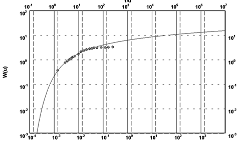
 Fig. 14.2. Matching the field data with the Theis Type Curve.

 

14.2.3 Cooper-Jacob Straight-Line Method for Time-Drawdown Data

The Cooper-Jacob equation [Eqn. (11.11)] expresses drawdown (s) as a linear function of ln(t) or log(t) if the limiting condition (u ≤ 0.01) is satisfied. This can be true for the large values of t and/or small values of r. Thus, the straight-line plot of drawdown (s) versus time (t) on the semi-logarithmic paper can occur after sufficient time has elapsed since the start of pumping. In case of multiple observation wells, the closer observation wells will meet the conditions earlier than the more distant ones.

 

The step-by-step procedure for determining confined aquifer parameters from time-drawdown data by the Cooper-Jacob straight-line method is as follows:

Step 1: Plot a field-data curve (s versus t) on the semi-logarithmic graph paper with the time on the X-axis (logarithmic scale) and the drawdown on the Y-axis (arithmetic scale).

Step 2: Fit a straight line to the field-data points.

Step 3: Extend the fitted straight line backward to intercept the zero-drawdown line and designate this time t_o.

Step 4: Compute the change in the value of the drawdown per log cycle (i.e., ∆s) from the slope of the straight line.

Step 5: Finally, compute the values of T and S by using the following equations:

 

                                                                                       (14.3)

 

and                                                                              (14.4)

 

14.2.4 Illustrative Example 2

Problem: To demonstrate the application of the Cooper-Jacob straight-line method, let’s consider the same problem as mentioned in Illustrative Example 1. In the present case, we have to calculate transmissivity (T) and storage coefficient (S) of the confined aquifer at 45 m location by the Cooper-Jacob straight-line method.     

 

Solution: Following the step-by-step procedure of the Cooper-Jacob straight-line method, a graph of drawdown versus log(t) is prepared and a straight line is fitted through the data points (after eliminating the data that considerably deviate from the straight line) as shown in Fig. 14.3.  

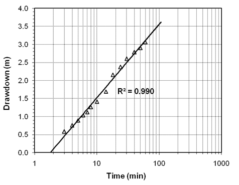
Fig. 14.3. Illustration of the Cooper-Jacob straight-line method.

 

From the graph, we have t₀ (time corresponding to the zero drawdown) = 1.8 min, and ∆s (drawdown per log cycle) = 3.55−1.5 = 2.05 m. Therefore, transmissivity (T) of the confined aquifer is:

 

Now, storage coefficient (S) of the confined aquifer is:

  

Check:

 

Since in the maximum value of u is larger than 0.01 (validity criterion of the Cooper-Jacob straight-line method), the Cooper-Jacob straight-line method is not strictly applicable to the present problem. Nevertheless, in this example, the value of S obtained by the Cooper-Jacob straight-line method is quite comparable with that yielded by the Theis Type Curve method, but the value of T is overestimated by the Cooper-Jacob straight-line method.  

 

14.2.5 Cooper-Jacob Straight-Line Method for Distance-Drawdown Data

If the drawdown is measured at the same time in several observation wells, it is found to vary with the distance from the pumping well in accordance with the Theis equation. If simultaneous measurements of the drawdown are made at a given time in three or more observation wells, the Cooper-Jacob straight-line method for time-drawdown data can be used after a minor modification. For example, let’s assume that two observation wells are located at distances r₁ and r₂ from the pumping well where drawdowns are measured at some time t as s₁ and s₂, respectively. Using the Cooper-Jacob equation [Eqn. (11.11b)], we have:

 

                                         (14.5)

 

and 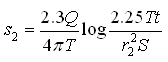                                                                                  (14.6)

 

From Eqns. (14.5) and (14.6), we have:

 

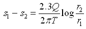                                                  (14.7)

 

Now, the Cooper-Jacob straight-line method described in Section 14.2.2 can be used as follows to determine confined aquifer parameters from the distance-drawdown data:

Step 1: Plot a drawdown (s) versus distance (r) field-data curve on the semi-logarithmic graph paper. Distance is plotted as a logarithmic scale on the X-axis, and drawdown is plotted on a linear scale on the Y-axis.

Step 2: Fit a straight line to the field-data points.

Step 3: Extend the fitted straight line to intercept the zero-drawdown line and designate this distance r₀.

Step 4: Calculate the change in the value of the drawdown per log cycle (i.e., ∆s) from the slope of the straight line.

Step 5: Finally, calculate the values of T and S by using the following equations:

 

                                                           (14.8)     

 

and                                                                                                  (14.9)

 

It should be noted that t in Eqn. (14.9) denotes a specific time since the start of pumping when the drawdowns are measured in multiple observation wells located in one direction at varying distances from the pumping well. These unsteady distance-drawdown data can yield both T and S. However, if instead of unsteady drawdowns steady or quasi-steady drawdowns are measured in multiple observation wells, the Thiem method can be directly used to calculate only T from such distance-drawdown data. The Thiem equation is applied for each pair of the steady (or quasi-steady) distance-drawdown data to obtain T values and then the mean of the T values is calculated which is taken as a representative aquifer parameter.     

 

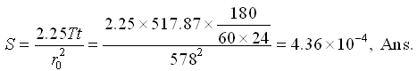
14.2.6 Illustrative Example 3

Problem: During a pumping test conducted in a confined aquifer, the aquifer was pumped at a constant rate of 280 m³/h. After 180 minutes of pumping, drawdowns were simultaneously measured in nine observation wells located at different radial distances from the pumping well as shown in Table 14.3.     Using the observed distance-drawdown data, determine transmissivity (T) and storage coefficient (S) of the confined aquifer.

 

 

Table 14.3. Unsteady Distance-Drawdown data

Distance (m)	3	15	30	45	60	75	90	120	150
Drawdown (m)	10.73	7.42	6.00	5.17	4.58	4.13	3.76	3.18	2.73

 

Solution: Following the procedure of the Cooper-Jacob straight-line method for distance-drawdown data mentioned above, a graph of drawdown versus log(r) is prepared and a straight line is fitted through the data points as shown in Fig. 14.4. 

 

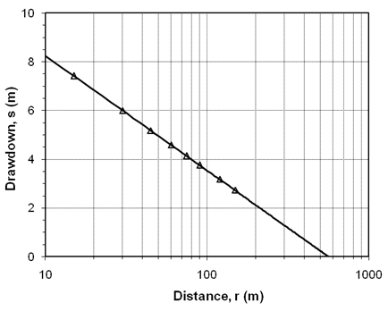
 Fig. 14.4. Straight-line fitting to the distance-drawdown data.

 

From the graph, we have r₀ (distance corresponding to the zero drawdown) = 578 m, and ∆s (drawdown per log cycle) = 8.25−3.5 = 4.75 m. Therefore, transmissivity (T) of the confined aquifer is:

 

Now, storage coefficient (S) of the confined aquifer is:

  

14.2.7 Residual Drawdown-Time Ratio Method for Recovery Data

To calculate the behavior of an aquifer after pumping has been stopped, i.e., during recovery phase, an imaginary recharging well with the same constant flow rate is superimposed on the pumping well, which is supposed to continue production (i.e., pumping) at the same constant rate. Thus, the two flow rates cancel each other, and in essence represent an idle well. As mentioned in Lesson 13, recovery test can be conducted either in the pumping well itself or in nearby observation wells. The analysis of recovery data obtained from pumping wells can yield only T or K not the storage coefficient (S) because of significant well losses in pumping wells. However, the analysis of recovery data obtained from observation wells can yield both T (or K) and S.

 

If t is the time since pumping starts and t¢ is the time since pumping stops, the residual drawdown (s¢) (Fig. 14.5) in a confined aquifer at any time (t’) after the end of pumping (i.e., during recovery period) can be obtained from the principle of superposition as follows:

 

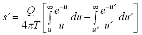                          (14.10)

 

Where,                 

                                                                  (14.11)

 

and                                                                                        (14.12)

 

 

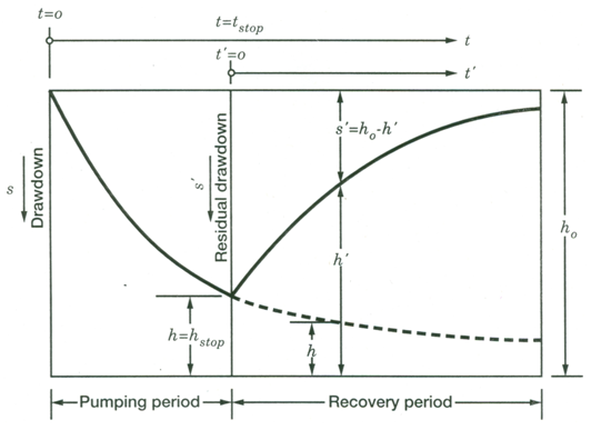
  Fig. 14.5. Schematic diagram of the aquifer recovery after the pump is turned off. (Source: Batu, 1998)

 

Since recovery measurements are made in a pumping well or in a nearby observation well, the value of r (distance of the measurement point from the pumping well) is normally small. A small value of r generally leads to a small value of u¢, which enables us to take advantage of the Cooper-Jacob approximation of the Theis well function. Applying the Cooper-Jacob assumption, Eqn. (14.10) reduces to:

 

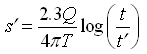                                         (14.13)

 

From Eqn. (14.13), transmissivity (T) can be calculated as:

 

                                  (14.14)

 

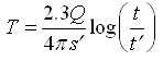
The step-by-step procedure for determining transmissivity and storage coefficient using recovery data is as follows:

Step 1: Plot a residual drawdown (s¢) versus time ratio (t/t¢) curve on the semi-logarithmic graph paper with the time ratio on the X-axis (logarithmic scale) and the residual drawdown on the Y-axis (arithmetic scale).

Step 2: Fit a straight line to the field-data points.

Step 3: Calculate the value of the residual drawdown per log cycle (∆s’) from the slope of the straight line.

Step 4: Calculate the transmissivity (T) as:

 

                                          (14.15)

 

As mentioned above, Storage coefficient (S) can be calculated only when the recovery data are measured in an observation well. The drawdown (s_p) when pumping is stopped at time (t_p) can be expressed as:

 

 

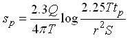                                  (14.16)

 

Once T is known from Eqn. (14.15), the storage coefficient (S) is calculated as:

 

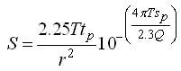                                (14.17)

 

14.2.8 Illustrative Example 4

Problem (Modified from Schwartz and Zhang, 2003): A pumping test was conducted in a confined aquifer and drawdowns were measured during both pumping period and recovery period in the pumping well (Table 14.4) as well as in an observation well (Table 14.5). In Tables 14.4 and 14.5, the first column contains the time since the pumping started (t), the second column contains the drawdown (s) during the pumping period, the third column contains the time since pumping stopped (t’), the fourth column contains the time ratio (t/t’), and the last column contains the residual drawdown (s’) during the recovery period.

 

Table 14.4. Time-Drawdown and Time-Residual Drawdown data from a pumping well (Source: Modified from Schwartz and Zhang, 2003)

t (min)	s (m)	t¢(min)	t/t¢	s¢(m)
20	3.44	20	41.00	0.46
80	3.54	80	11.00	0.30
140	3.60	140	6.71	0.24
195	3.60	195	5.10	0.21
255	3.60	255	4.14	0.18
315	3.66	315	3.54	0.16
375	3.72	375	3.13	0.15
435	3.72	435	2.84	0.14
495	3.72	495	2.62	0.12
560	3.72	560	2.43	0.10
616	3.75	616	2.30	0.10
668	3.78	668	2.12	0.10
737	3.81	737	2.10	0.07
800	3.81	800	2.00	0.07

 

Table 14.5. Time-Drawdown and Time-Residual Drawdown data from an observation well (Source: Modified from Schwartz and Zhang, 2003)

t (min)	s (m)	t¢(min)	t/t¢	s¢(m)
5	0.02	5	161.00	0.54
10	0.07	10	81.00	0.50
15	0.10	15	54.33	0.47
20	0.12	20	41.00	0.44
25	0.15	25	33.00	0.42
30	0.17	30	27.67	0.40
40	0.20	40	21.00	0.37
50	0.22	50	17.00	0.35
60	0.24	60	14.33	0.33
70	0.26	70	12.43	0.31
80	0.28	80	11.00	0.30
90	0.29	90	9.89	0.29
100	0.30	100	9.00	0.27
110	0.32	110	8.27	0.27
120	0.33	120	7.67	0.26
180	0.38	180	5.44	0.21
240	0.41	240	4.33	0.19
300	0.44	300	3.67	0.16
360	0.46	360	3.22	0.15
420	0.48	420	2.90	0.14
480	0.50	480	2.67	0.12
540	0.52	540	2.48	0.11
600	0.53	600	2.33	0.11
660	0.54	660	2.21	0.10
720	0.55	720	2.11	0.09
800	0.57	800	2.00	0.09

 

A constant pumping rate of 270 m³/h was maintained during the pumping period. The observation well was situated 22 m away from the pumping well. Determine hydraulic parameters of the confined aquifer using the above two sets of the recovery data.

 

Solution: Residual drawdown (s¢) and time ratio (t/t¢) data obtained from the pumping well and the observation well were plotted on the semi-logarithmic graph paper as illustrated in Figs. 14.6 and 14.7, respectively. Thereafter, a straight line was fitted to the residual drawdown versus time ratio curve in each figure. After selecting two suitable points on each graph as indicated in Figs. 14.6 and 14.7, we have Ds¢= 0.43 − 0.13 = 0.30 m in the pumping well from Fig. 14.6 and Ds¢= 0.53 − 0.28 = 0.25 m in the observation well from Fig. 14.7. From the question, pumping rate (Q) = 270 m³/h. Given these data, the transmissivity (T) of the confined aquifer can be determined from the recovery data of the pumping well as:

 

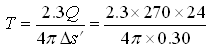 = 3953.41 m²/day, Ans.

 

As we know that the storage coefficient (S) cannot be determined from the recovery data of the pumping well.

 

Similarly, the transmissivity (T) of the confined aquifer can be determined from the recovery data of the observation well as:

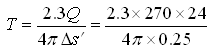 = 4744.09 m²/day, Ans.

 

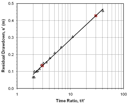
Fig. 14.6. Straight-line fitting to the residual drawdown-time ratio data obtained from the pumping well.

  

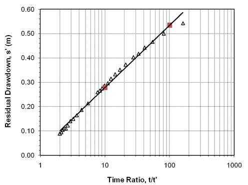
Fig. 14.7. Straight-line fitting to the residual drawdown-time ratio data obtained from the observation well.

 

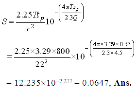
Now, from the question we have: t_p = 800 min, s_p = 0.57 m (Table 14.5), Q = 270 m³/h = 270/60 = 4.5 m³/min, r = 22 m, and T = 4744.09 m²/day = 4744.09/(24´60) = 3.29 m²/min as computed above. Using these data, the storage coefficient (S) of the confined aquifer can be determined as:

  

14.2.9 Cooper-Jacob Straight-Line Method for Recovery Data

The Cooper-Jacob straight-line method can be used to analyze the time-recovery data obtained from a pumping well or an observation well. The step-by-step procedure for analyzing time-recovery data by the Cooper-Jacob straight-line method is the same as that for analyzing the time-drawdown data described in Section 14.2.3, except that the time is measured since pumping stopped (Fig. 14.5), and ‘recovery’ is used instead of drawdown. Finally, Eqn. (14.3) is used to determine T and Eqn. (14.4) is used to determine S from the time-recovery data. In this case also, storage coefficient (S) cannot be determined using the time-recovery data obtained from a pumping well.

 

Note that ‘recovery’ is calculated as the difference between the extrapolated time-drawdown curve and the ‘residual drawdown’ (Fig. 14.5). Residual drawdown at time t after the pump is turned off is the difference between the static groundwater level (i.e., pre-pumping groundwater level) and the depth of groundwater at time t.

 

14.3 Determination of Unconfined Aquifer Parameters

14.3.1 Unconfined Aquifer without Delayed Yield

The methods mentioned above for confined aquifers are also applicable to the unconfined aquifers exhibiting no delayed yield. However, in this case, it is necessary to check whether correction in the observed drawdowns is required or not. This checking is done by using the following criteria:

 

Case A: If  0.02, then no correction in the observed drawdown is needed. Here, s_max = maximum drawdown at a given location during pumping test and h₀ = initial saturated thickness of the unconfined aquifer. Therefore, the observed time-drawdown data of unconfined aquifers as such can be used for determining unconfined aquifer parameters (K and S_y) by the Theis Type-Curve method, the Cooper-Jacob Straight-Line method, or the methods for analyzing recovery data.

 

After determining T (transmissivity) and S (storage coefficient) from any of the above methods, the hydraulic conductivity (K) of the unconfined aquifer can be obtained by dividing T with initial saturated thickness of the unconfined aquifer (h₀). The value of S will be equal to the specific yield (S_y) of the unconfined aquifer. Thus, K and S_y of unconfined aquifers can be determined from time-drawdown pumping-test data. Also, the Thiem method can be used for determining T or K from steady or quasi-steady distance-drawdown data.

 

Case B: If  > 0.02, then the observed drawdown must be corrected using Eqn. (14.18) in order to obtain drawdowns in the equivalent confined aquifer so that the methods used for confined aquifers can be applicable to unconfined aquifers as well.

 

                                            (14.18)

 

Where, = corrected drawdown (i.e., drawdown in the equivalent confined aquifer), s = drawdown measured in the unconfined aquifer, and h₀ = initial saturated thickness of the unconfined aquifer.

 

After correcting the observed/measured drawdowns of the unconfined aquifer, the corrected time-drawdown data can be used to determine unconfined aquifer parameters (K and S_y) by the Theis Type-Curve method, the Cooper-Jacob Straight-Line method, or the methods for analyzing recovery data as mentioned in Case A above. Similarly, the Thiem method can be used for determining T or K of unconfined aquifers from steady or quasi-steady distance-drawdown data measured in unconfined aquifers.

 

14.3.2 Unconfined Aquifer with Delayed Yield

If the time-drawdown data obtained from unconfined aquifers exhibit significant delayed yield, the above-mentioned methods cannot be used for determining aquifer parameters. In this case, different methods have been suggested for reliable results which are: (i) Type-Curve Method, and (ii) Neuman Straight-Line Method. Excellent descriptions of these methods can be found in Fetter (1994), Schwartz and Zhang (2003) and Batu (1998).

 

14.4 Identification of Aquifer Boundaries

A common field problem is to identify and locate aquifer boundaries. Pumping-test data can provide quantitative answers to this problem by the application of image well theory and unsteady (transient) flow equations. As discussed in Lesson 13, if a pumping well and an observation well are located near an unknown impermeable aquifer boundary, the real pumping well and the image well are considered to be operating simultaneously and the drawdowns caused by the real and image pumping wells are additive, resulting in an effective discharge boundary of no flow. When determining the distance to a barrier boundary, the image well is assumed to pump water out of the aquifer at the same rate as the water is withdrawn by the real pumping well. Similarly, when estimating the distance to a recharge boundary, the image well is assumed to inject water into the aquifer at the same rate as water is withdrawn by the real pumping well. Thus, the resulting drawdown caused by the real pumping well and simulated ‘build up’ of water caused by the recharging image well equals an effective recharge boundary with zero drawdown in the aquifer.

 

According to the law of times, the time of occurrence of zero drawdown or equal drawdown is directly proportional to the square of the distances of the observation wells from the pumping well and is independent of the rate of pumping. That is,

 

                                                 (14.19)

 

Where, r = distance of the observation well from the real well (pumping well), r_i = distance of the observation well from the image well, t_p = time since pumping started to any selected drawdown before the boundary influences the well drawdown (Fig. 14.8), and t_i = time since pumping started where the divergence of the time-drawdown curve from the Type curve equals the selected drawdown (Fig. 14.8).

 

The value of r_i can be obtained from Eqn. (14.19) and half the value is taken approximately as the distance of the aquifer boundary from the pumping well.

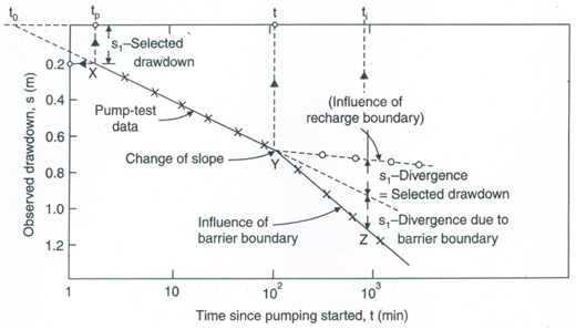
Fig. 14.8. Identification of aquifer boundaries using semi-logarithmic plot of time-drawdown data. (Source: Raghunath, 2007)

 

Alternatively, if the time t₀ corresponding to the zero drawdown is selected from the Cooper-Jacob’s time-drawdown curve and t is the time at which a change of slope (i.e., divergence) is indicated (Fig. 14.8), the distance of the aquifer boundary from the pumping well can be obtained from the following equation: 

 

                                                 (14.20)

 

It should be noted that the distance r_i obtained from Eqn. (14.19) or Eqn. (14.20) gives an arc on which the image well lies. Data from two or more observation wells are required to locate the image well from the intersection of the three arcs (Fig. 14.9). Then, the location of the aquifer boundary is found to be midway and perpendicular to the line joining the pumping well and the image well as shown in Fig. 14.9.

  

 

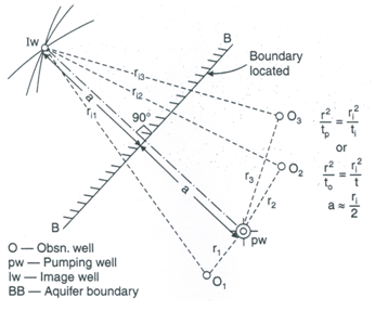
Fig. 14.9. Finding the location of an aquifer boundary.

(Source: Raghunath, 2007)

 

References

• Batu, V. (1998). Aquifer Hydraulics: A Comprehensive Guide to Hydrogeologic Data Analysis. John Wiley & Sons, New York.

• Fetter, C.W. (1994). Applied Hydrogeology. Third Edition, Prentice Hall, NJ.

• Kasenow, M. (2001). Applied Groundwater Hydrology and Well Hydraulics. Second Edition, Water Resources Publications, Highlands Ranch, Colorado.

• Kruseman, G.P. and de Ridder, N.A. (1994). Analysis and Evaluation of Pumping Test Data. Second Edition, ILRI Publication 47, International Institute for Land Reclamation and Improvement (ILRI), Wageningen, The Netherlands.

• Michael, A.M., Khepar, S.D. and Sondhi, S.K. (2008). Water Well and Pump Engineering. Second Edition, Tata McGraw Hill Education Pvt. Ltd., New Delhi.

• Raghunath, H.M. (2007). Ground Water. New Age International (P) Limited, New Delhi.

• Roscoe Moss Company (1990). Handbook of Ground Water Development. John Wiley & Sons, New York.

• Samuel, M.P. and Jha, M.K. (2003). Estimation of aquifer parameters from pumping test data by genetic algorithm optimization technique. Journal of Irrigation and Drainage Engineering, ASCE, 129(5): 348-359.

• Schwartz, F.W. and Zhang, H. (2003). Fundamentals of Ground Water. John Wiley & Sons, New York.

 

Suggested Readings

• Fetter, C.W. (2000). Applied Hydrogeology. Fourth Edition. Prentice Hall, NJ.

• Schwartz, F.W. and Zhang, H. (2003). Fundamentals of Ground Water. John Wiley & Sons, New York.

• Kasenow, M. (2001). Applied Groundwater Hydrology and Well Hydraulics. Second Edition, Water Resources Publications, Highlands Ranch, Colorado.

• Raghunath, H.M. (2007). Ground Water. New Age International (P) Limited, New Delhi.

• Michael, A.M., Khepar, S.D. and Sondhi, S.K. (2008). Water Well and Pump Engineering. Second Edition, Tata McGraw Hill Education Pvt. Ltd., New Delhi.