Watershed Hydrology 3(2+1)

Lesson 6 Presentation of Rainfall Data

6.1 Mass Curve of Rainfall

The mass curve of rainfall is a plot of the accumulated precipitation against time,plotted in chronological order. Records of float type and weighing-bucket typegauges are of this form. A typical mass curve of rainfall at a station during a storm is shown in fig 6.1. Mass curves of rainfall are very useful in extractingthe information on the duration and magnitude of astorm. Also, intensities atvarious time intervals in a storm can be obtained by the slope of the curve.Fornon-recording raingauges, mass curves are prepared from knowledge of theapproximate beginning and end of a storm and by using the mass curves ofadjacent recording gauge stations as a guide

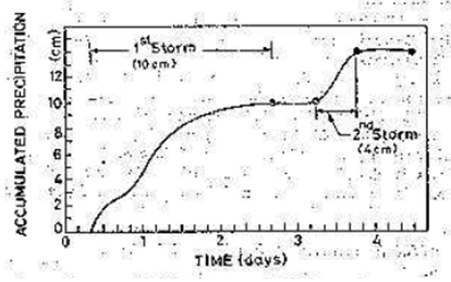
Fig. 6.1.Mass curve of rainfall.(Source: Subramanya, 2006)

6.2 Hyetograph

A hyetograph is a plot of the intensity of rainfall against the time in the hyetograph is derived from the mass curve and is usually represented as a bar chart (Fig. 6.2). It is a very convenient way of represents characteristics of a storm and is particularly important in thedevelopment of a design storms to predict extreme floods. The area under a hyetograph represents the total precipitation received in that period. The time in used depends on the purpose; in urban-drainage problems small durations are used while in flood-flow computations in larger catchments the intervals are of about 6 hours.

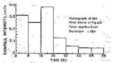
Fig. 6.2.Hyetograph of a storm.(Source: Subramanya, 2006)

 

6.3 Depth-Area-Duration Relationships

The areal distribution characteristics of a storm of given duration is reflected in its depth-area-relationship.

 

6.3.1 Depth-Area Relation

For a rainfall of a given duration, the average depth decreases with the area in an exponential fashion given by

Where,  is average depth in cms over an area A km²,is highest amount ofrainfall in cm at the storm centre and K and n are constant for a given region.

On the basis of 42 severe most storms in north India, Dhar and Bhattacharya(1975) have obtained the following values for K and n for storms of different duration.

Duration	K	n
1 day	0.0008526	0.6614
2 days	0.0009877	0.6306
3 days	0.0017454	0.5961

 

Since it is very unlikely that the storm centre coincides over a raingauge station, the exact determination of  is not possible. Hence in the analysis of large area storms the highest station rainfall is taken as the average depth over an area of 25 km².

 

6.3.2 Maximum Depth-Area-Duration Curves

In many hydrological studies involving estimation of severe floods, it is necessary to have information on the maximum amount of rainfall of various duration occurring over various sizes of areas. The development of relationship, between maximum depth-area-duration for a region is known as DAD analysis and forms an important aspect of hydro-meteorological study. A brief description for the DAD analysis is given below.

 

First the severe most rainstorms that have occurred in the region in the question are considered. Isohyetal maps and mass curves of the storm are compiled. A depth area curve of a given duration of the storm is prepared. Then from a study of the mass curve of rainfall, various durations and the maximum depth of rainfall in these durations are noted. The maximum depth-area curve for a given duration D is prepared by assuming the area distribution of rainfall for smaller duration to be similar to the total storm. The procedure is then repeated for different storms and the envelope curve of maximum depth-area for duration D is obtained. A similar procedure for various values of D results in a family of envelopes curve of maximum depth vs area, with duration as the third parameter (Fig 6.3).These curves are called DAD curves.

 

Fig 6.3 shows typical DAD curves for a catchment. In this the average depth denotes the depth averaged over the area under consideration. It may be seen that the maximum depth for a given storm decreases with the area; for a given area the maximum depth increases with the duration.

 Preparation of DAD curves involves considerable computational effort and requires meteorological and topographical information of the region. Detailed data on severe most storms in the past are needed. DAD curves are essential to develop design storms for use in computing the design flood in the hydrological design of major structures such as dams. 

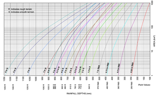
Fig. 6.3.Typical DAD Curves. (Source: Raghunath, 2006)

 

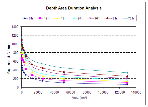
Solved Example

Construct maximum depth-area-duration curve for the data given below:

Area (km2)	Maximum rainfall (mm)*
	Duration (h)
	6	12	18	24	36	48	72
25	635	765	930	991	1070	1103	1156
258	506	676	834	902	971	996	1039
517	463	658	806	877	940	966	1004
1294	399	633	802	839	897	922	955
2589	348	582	704	775	844	864	894
5179	292	423	580	638	701	729	762
12945	214	290	366	402	483	534	628
25895	153	209	265	315	392	450	549
51795	110	160	209	252	303	359	455
129495	72	115	143	168	209	259	343
258995	51	72	97	117	160	176	234

 

 

References

Subramanya, K. (2006). Engineering Hydrology. Tata McGraw-Hill publishing company Limited,32-38.

Raghunath, H.M. (2006). Hydrology. New Age International (P) Ltd., 18-21.

Suggested Readings

Singh, V. P. (1994). Elementary Hydrology. Prentice Hall of India Private Limited, New Delhi.

Suresh R. (2007). Soil and Water Conservation Engineering.Fourth edition, Standard Publishers Distributors, New Delhi.