Watershed Hydrology 3(2+1)

Lesson 9 Estimation of Mean Areal Rainfall

1. Arithmetic or Station Average Method

2. Thiessen Polygon Method

3. Isohyetal Method.

 

9.1            Arithmetic Average Method

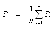
This method consists of computing the arithmetic average of the values of the precipitation for all stations within the area.  Since this method assigns equal weight to all stations irrespective of their relative location and other factors, it should be adopted in area where rainfall is uniformly distributed.

 

                                                                                              (9.1)                      

Where average precipitation is over an area, P is the precipitations at individual station i, and n is the number of stations.

 

 

9.2            Thiessen Polygon Method

This is a graphical technique which calculates station weights based on the relative areas of each measurement station in the Thiessen polygon network.Rainfall varies in intensity and duration from one place to other; hence rainfall recorded by each station should be weighed according to the area (polygons) it is assumed to influence. The individual weights are multiplied by the station observation and the values are summed to obtain the areal average precipitation.This method is useful for areas, which are more or less plain and are of intermediate size (500 to 5000 km²).   This method is also used when there are a few raingage stations compared to size.  The polygons are formed as follows:

1. The stations are plotted on a map of the area drawn to a scale.

2. The adjoining stations are connected by the dashed lines.

3. Perpendicular bisectors are constructed on each of these dashed lines.

4. These bisectors form polygons around each station (effective area for the station within the polygon).  For stations close to the boundary, the boundary lines form the closing limit of the polygons.

 

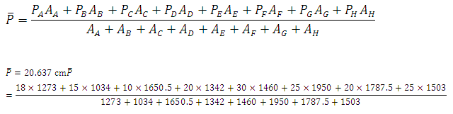
Area of each polygon (A_i)is determined and the average precipitation is calculated using the following equation:

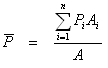        (9.2) Where A is the total area of the watershed.

 

9.3            Isohyetal Method

This is a graphical technique which involves drawing estimated lines of equal rainfall over an area based on point measurements. Then multiply the area between each contour by the average precipitation in the area to get the rainfall volume in the area. Sum these volumes to get the total rainfall volume, and then divide the total rainfall volume by the area of the watershed to get the average areal precipitation in the watershed.

 

Let’s take it step by step:

Step1: Determine what contours of equal precipitation (called isohytes) you will use.

This varies from situation to situation, but you want to have as many contours as necessary to get an accurate model, but not so many that your construction becomes cluttered. 

Step2: Draw a line between gauges that will be separated by isohyets. 

Step3: Plot points on those lines that correspond to the isohyets determined in Step 2. 

Step4: Now sketch the isohyets. 

Step5: Redraw the construction onto graph paper with the isohyetal lines. Then count the boxes between each of the isohyetal lines. 

Step6: Find the actual watershed area between each isohyet. These areas will be lettered starting with A at the top and moving alphabetically toward the bottom of the construction. 

Step7: Multiply the areas found in Step 6 by the average precipitation in the area. 

Step8: Divide the sum of the values found in Step 7 by the total area of the watershed to get the average rainfall in the area.

 

9.4 Raingage Network

There is no single answer to determining the mean areal rainfall because it is affected by so many factors. However, the denser the gage network, the more accurate is the representation.  Gages are not evenly spaced, high variability areas have more gages and relatively uniform rainfall areas have fewer gages.  In addition, costs of installation, maintenance of the network, as well as its accessibility to the observer, are also important consideration.

 

In general, the sampling errors of rainfall tends to increase with increasing mean areal rainfall, and decrease with increasing network density, duration of rainfall, and areal extend.  Accordingly, larger average errors are produced by a particular network for storm rainfall than for monthly, seasonal or annual rainfall.

 

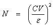
The adequacy of an existing rain-gage network of a watershed is assessed statistically.  The optimum number of raingages corresponding to an assigned percentage of error in estimation of mean areal rainfall can be obtained as:

 

                     (9.3)                                                        

Where, N is the optimum number of raingages, CV is the coefficient of variation of the rainfall values of the gages, and  is the assigned percentage of error in estimation of mean areal rainfall.

                                                           (9.4)         

In which  is the mean rainfall defined as

 

           

                                                                  

and S is the standard deviation of rainfall computed as

 

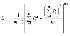                          (9.6)                            

Where, m is the number of raingages in the watershed recording P₁, P₂,…, P_m values of rainfall for fixed time interval.  Generally, value of   is taken as 10%.

 

Example: A catchment has six raingage stations.  In a year, the annual rainfalls recorded by the gages are as follows:

 

Stations      :       A       B       C       D       E       F

Rainfall (cm):       82.6   102.9 180.3 110.3 98.8   136.7

 

For a 10% error in the estimation of mean rainfall, calculate optimum number of stations in the catchment.

 

Solution:

Number of stations (m) = 6,

Mean precipitation =118.6 cm

Standard deviation of precipitation (S) = 35.04

Error  (ε)    =10%

=29.54 

              

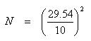 = 8.7 =    9      stations

 

9.4.1 WMO Recommended Precipitation Network Density

• One station per 600 to 900 km² - in flat regions of temperate, Mediterranean and tropical zone.

• One station per 100 to 250 km² – in mountainous regions of temperate, Mediterranean and tropical zone.

• One station per 25 km² – in small mountainous land with irregular precipitation.

• One station per 1500 to 10,000 km² – arid and polar zones.

 

9.4.2 Indian Standard Recommendation

• One station per 520 km² - in plains.

• One station per 260-390 km²– in regions of average elevation of 1000 m.

• One station per 130 km²– in predominantly hilly areas with heavy rainfall.

 

 

Solved Problems

Example 1

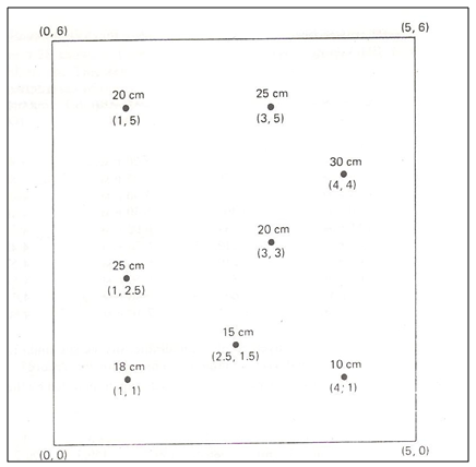
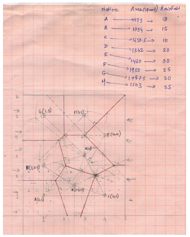
Estimate the mean areal rainfall for the area shown in Fig. 3.1, using the Thiessen polygon method.

 Answer

 

 

Example 2

A catchment area has seven raingauge stations. In a year the annual rainfall recorded by the gauges are as follows:

Station	P	Q	R	S	T	U	V
Rainfall (cm)	130.0	142.1	118.2	108.5	165.2	102.1	146.9

 

For a 5% error in the estimation of mean rainfall, calculate the minimum number of additional stations required to be established in the catchment.

Answer

	P	P-Pavg	(P-Pavg)2
P	130	-0.43	0.18
Q	142.1	11.67	136.18
R	118.2	-12.23	149.57
S	108.5	-21.93	480.92
T	165.2	34.77	1208.95
U	102.1	-28.33	802.58
V	146.9	16.47	271.26
MEAN	130.43		3049.67
Standard Deviation	20.87		22.54
			130.42
Coefficient of Variation
			0.17
Coefficient of Variation (%)			17.28
Percentage error (%)			5
Optimum number of rain gauge stations	12		11.95
Answer	12-7=5

 

 

 

 

References

• Subramanya, K. (2006). Engineering Hydrology. Tata McGraw-Hill Publishing Company Limited, 28-35.

Suggested Reading

• Singh, V. P. (1994). Elementary Hydrology. Prentice Hall of India Private Limited,New Delhi.