Watershed Hydrology 3(2+1)

Lesson 10 Frequency Analysis of Point Rainfall

10.1  Plotting Position Formulae

There are two methods for performing frequency analysis

• Empirical method

• Frequency factor method

The excedence probability of the event is obtained by the use of empirical formula, known as plotting position.

 

Several plotting position formulas were developed and some of them are given below:

  

Table 10.1. Plotting position formulae (Source: Subramanya, 2006)

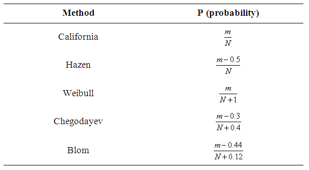
m = rank assigned to the data after arranging them in descending order of magnitude

Thus the maximum value is assigned m =1, the second largest value (m =2), and the lowest value m =N. 

N = number of records. 

 

Weibull formula is the most commonly used plotting position formula.

• Having calculated P and T for all the events in the series, the variation of rainfall magnitude is plotted against the corresponding T on semi-log or log-log paper.  

• The rainfall magnitude for any recurrence interval can be determined by extrapolating the plot between magnitude and recurrence interval. 

• Empirical procedures can give good results for small extrapolations but the errors increased with the amount of extrapolation.  

• For more accurate results, analytical methods using frequency factor are used.

 

Example

For a station A, the recorded annual 24 h maximum rainfall is given below.

Year	Rainfall (cm)	Year	Rainfall (cm)	Year	Rainfall (cm)
1950	13.0	1957	12.5	1964	8.5
1951	12.0	1958	11.2	1965	7.5
1952	7.6	1959	8.9	1966	6.0
1953	14.3	1960	8.9	1967	8.4
1954	16.0	1961	7.8	1968	10.8
1955	9.6	1962	9.0	1969	10.6
1956	8.0	1963	10.2	1970	8.3
				1971	9.5

 

(a)  Estimate the 24 h maximum rainfall with return periods of 13 and 50 years.

(b) What would be the probability of a rainfall of magnitude equal to or exceeding 10 cm occurring in 24 h at station A.

 

Solution

m	Rainfall, cm	P =m/n+1	T=1/P	m	Rainfall, cm	P =m/n+1	T=1/P
1	16	0.043	23.00	12	9	0.522	1.92
2	14.3	0.087	11.50	13	8.9
3	13	0.130	7.67	14	8.9	0.609	1.64
4	12.5	0.174	5.75	15	8.5	0.652	1.53
5	12	0.217	4.60	16	8.4	0.696	1.44
6	11.2	0.261	3.83	17	8.3	0.739	1.35
7	10.8	0.304	3.29	18	8	0.783	1.28
8	10.6	0.348	2.88	19	7.8	0.826	1.21
9	10.2	0.391	2.56	20	7.6	0.870	1.15
10	9.6	0.435	2.30	21	7.5	0.913	1.10
11	9.5	0.478	2.09	22	6	0.957	1.05

Rainfall Frequency Curve

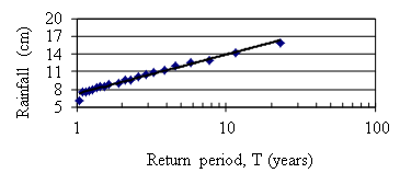
(a)  After interpolating and extrapolating the above graph, we can determine rainfall magnitude for 13 and 50 year return period respectively.

 

          13 year RI   = 14.55 cm

          50 year RI   = 18.00 cm

 

(b)  For Rainfall = 10 cm, T =2.4 years and P = 0.417.

 

10.2 Intensity-duration-frequency (IDF) Relationship

• In many studies related to watershed management, such as runoff disposal and erosion control, it is necessary to know the rainfall intensities of different durations and return periods.

 

• The relationship between intensity (i, cm/hr), duration (d, hour) and return period (T, years) can be expressed as follows:

 

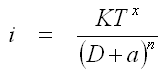                               (10.1)                            

Where K, x, a and n are constants for a given catchment.

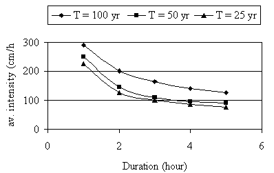
                             Intensity –Duration-Frequency Curve

 

Typical values of constants K,, x, a, and n for a few selected cities are given below:

Table – Values of constants in equation (29)

(Source: CSWCRTI- Dehradun)

City	K	x	A	n
Bhopal	6.93	0.189	0.50	0.878
Nagpur	11.45	0.156	1.25	1.032
Chandigarh	5.82	0.160	0.40	0.750
Bellary	6.16	0.694	0.50	0.972
Raipur	4.68	0.139	0.15	0.928

 

Example: Compute 10 year, 1 hour design rainfall intensity for Bhopal and Nagpur.

Solution:

For Bhopal

 

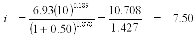          cm/hr

 

For Nagpur

 

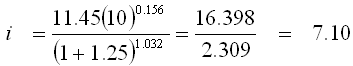          cm/hr

 

Example

Perform the frequency analysis using different graphical methods for the following annual rainfall data. Estimate annual rainfall amount with 100 and 50 years return periods.

Year	Annual rain (mm)	Year	Annual rain (mm)	Year	Annual rain (mm)
1950	115	1959	71.4	1968	68.6
1951	96.5	1960	83	1969	67
1952	78	1961	96.5	1970	93
1953	89.5	1962	88.3	1971	108.8
1954	94.7	1963	70.6	1972	104.2
1955	73.3	1964	84.5	1973	89
1956	79.3	1965	92.7	1974	86
1957	87.1	1966	101.8
1958	124.8	1967	76.4

 

Solution

Year	Annual rain (mm)	Data in Descending Order	Rank (m)	PCa= (m/N)	TCa= 1/Pca	PH = (m-0.5)/N	TH= 1/PH	PW= m/ (N+1)	TW= 1/PW
				California		Hazen		Weibull
1950	115	124.8	1	0.04	25.00	0.02	50.00	0.038	26.00
1951	96.5	115	2	0.08	12.50	0.06	16.67	0.077	13.00
1952	78	108.8	3	0.12	8.33	0.1	10.00	0.115	8.67
1953	89.5	104.2	4	0.16	6.25	0.14	7.14	0.154	6.50
1954	94.7	101.8	5	0.2	5.00	0.18	5.56	0.192	5.20
1955	73.3	96.5	6	0.24	4.17	0.22	4.55	0.231	4.33
1956	79.3	96.5	7	0.28	3.57	0.26	3.85	0.269	3.71
1957	87.1	94.7	8	0.32	3.13	0.3	3.33	0.308	3.25
1958	124.8	93	9	0.36	2.78	0.34	2.94	0.346	2.89
1959	71.4	92.7	10	0.4	2.50	0.38	2.63	0.385	2.60
1960	83	89.5	11	0.44	2.27	0.42	2.38	0.423	2.36
1961	96.5	89	12	0.48	2.08	0.46	2.17	0.462	2.17
1962	88.3	88.3	13	0.52	1.92	0.5	2.00	0.500	2.00
1963	70.6	87.1	14	0.56	1.79	0.54	1.85	0.538	1.86
1964	84.5	86	15	0.6	1.67	0.58	1.72	0.577	1.73
1965	92.7	84.5	16	0.64	1.56	0.62	1.61	0.615	1.63
1966	101.8	83	17	0.68	1.47	0.66	1.52	0.654	1.53
1967	76.4	79.3	18	0.72	1.39	0.7	1.43	0.692	1.44
1968	68.6	78	19	0.76	1.32	0.74	1.35	0.731	1.37
1969	67	76.4	20	0.8	1.25	0.78	1.28	0.769	1.30
1970	93	73.3	21	0.84	1.19	0.82	1.22	0.808	1.24
1971	108.8	71.4	22	0.88	1.14	0.86	1.16	0.846	1.18
1972	104.2	70.6	23	0.92	1.09	0.9	1.11	0.885	1.13
1973	89	68.6	24	0.96	1.04	0.94	1.06	0.923	1.08
1974	86	67	25	1	1.00	0.98	1.02	0.962	1.04

Year	Annual rain (mm)	Data in Descending Order	Rank (m)	PCh= (m-0.3)/(N+0.4)	TCh = 1/PCh	PB= (m-0.44)/(N+0.12)	TB= 1/PB	PG= (m-3/8)/(N+1/4)	TG= 1/PG
				Chegodayev		Blom		Gringorten
1950	115	124.8	1	0.03	36.29	0.02	44.86	0.02	40.40
1951	96.5	115	2	0.07	14.94	0.06	16.10	0.06	15.54
1952	78	108.8	3	0.11	9.41	0.10	9.81	0.10	9.62
1953	89.5	104.2	4	0.15	6.86	0.14	7.06	0.14	6.97
1954	94.7	101.8	5	0.19	5.40	0.18	5.51	0.18	5.46
1955	73.3	96.5	6	0.22	4.46	0.22	4.52	0.22	4.49
1956	79.3	96.5	7	0.26	3.79	0.26	3.83	0.26	3.81
1957	87.1	94.7	8	0.30	3.30	0.30	3.32	0.30	3.31
1958	124.8	93	9	0.34	2.92	0.34	2.93	0.34	2.93
1959	71.4	92.7	10	0.38	2.62	0.38	2.63	0.38	2.62
1960	83	89.5	11	0.42	2.37	0.42	2.38	0.42	2.38
1961	96.5	89	12	0.46	2.17	0.46	2.17	0.46	2.17
1962	88.3	88.3	13	0.50	2.00	0.50	2.00	0.50	2.00
1963	70.6	87.1	14	0.54	1.85	0.54	1.85	0.54	1.85
1964	84.5	86	15	0.58	1.73	0.58	1.73	0.58	1.73
1965	92.7	84.5	16	0.62	1.62	0.62	1.61	0.62	1.62
1966	101.8	83	17	0.66	1.52	0.66	1.52	0.66	1.52
1967	76.4	79.3	18	0.70	1.44	0.70	1.43	0.70	1.43
1968	68.6	78	19	0.74	1.36	0.74	1.35	0.74	1.36
1969	67	76.4	20	0.78	1.29	0.78	1.28	0.78	1.29
1970	93	73.3	21	0.81	1.23	0.82	1.22	0.82	1.22
1971	108.8	71.4	22	0.85	1.17	0.86	1.17	0.86	1.17
1972	104.2	70.6	23	0.89	1.12	0.90	1.11	0.90	1.12
1973	89	68.6	24	0.93	1.07	0.94	1.07	0.94	1.07
1974	86	67	25	0.97	1.03	0.98	1.02	0.98	1.03

 

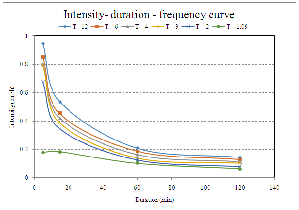
Example

Develop intensity-duration-frequency curve for given data

5 min		15 min		60 min		120 min
Year	Rainfall	Year	Rainfall	Year	Rainfall	Year	Rainfall
	mm		mm		mm		mm
1908	0.79	1910	1.34	1916	2.09	1917	2.91
1910	0.71	1914	1.13	1914	1.87	1914	2.58
1918	0.67	1916	1.05	1910	1.64	1911	2.28
1914	0.66	1918	0.97	1915	1.39	1908	2.06
1916	0.6	1909	0.91	1908	1.34	1916	1.77
1912	0.56	1913	0.86	1912	1.27	1913	1.58
1917	0.45	1915	0.84	1918	1.19	1910	1.49
1915	0.39	1917	0.76	1917	1.14	1909	1.45
1913	0.3	1911	0.61	1909	1.08	1912	1.4
1911	0.22	1912	0.56	1911	1.05	1915	1.35
1909	0.15	1908	0.46	1913	1.03	1918	1.28

 

Solution

5 min		15 min		60 min		120 min
Year	Rainfall Intensity	Year	Rainfall Intensity	Year	Rainfall Intensity	Year	Rainfall Intensity
	cm/h		cm/h		cm/h		cm/h
1908	0.948	1908	0.536	1908	0.209	1915	0.1455
1921	0.852	1915	0.452	1904	0.187	1908	0.129
1915	0.804	1904	0.42	1915	0.164	1904	0.114
1934	0.792	1921	0.388	1926	0.139	1921	0.103
1929	0.72	1926	0.364	1921	0.134	1926	0.0885
1926	0.672	1934	0.344	1914	0.127	1917	0.079
1931	0.54	1929	0.336	1931	0.119	1914	0.0745
1904	0.468	1931	0.304	1934	0.114	1931	0.0725
1917	0.36	1911	0.244	1929	0.108	1934	0.07
1914	0.264	1917	0.224	1911	0.105	1929	0.0675
1911	0.18	1914	0.184	1917	0.103	1911	0.064

 

 

For 5 min duration
Year	Rainfall	Rainfall Intensity	Rank	P= (m/(n+1))	T= (1/P)
	mm	cm/h
1908	0.79	0.948	1	0.0833	12.00
1921	0.71	0.852	2	0.1667	6.00
1915	0.67	0.804	3	0.2500	4.00
1934	0.66	0.792	4	0.3333	3.00
1929	0.6	0.72	5	0.4167	2.40
1926	0.56	0.672	6	0.5000	2.00
1931	0.45	0.54	7	0.5833	1.71
1904	0.39	0.468	8	0.6667	1.50
1917	0.3	0.36	9	0.7500	1.33
1914	0.22	0.264	10	0.8333	1.20
1911	0.15	0.18	11	0.9167	1.09

 

For 15 min duration
Year	Rainfall	Rainfall Intensity	Rank	P= (m/(n+1))	T= (1/P)
	mm	cm/h
1908	1.34	0.536	1	0.0833	12.00
1921	1.13	0.452	2	0.1667	6.00
1915	1.05	0.42	3	0.2500	4.00
1934	0.97	0.388	4	0.3333	3.00
1929	0.91	0.364	5	0.4167	2.40
1926	0.86	0.344	6	0.5000	2.00
1931	0.84	0.336	7	0.5833	1.71
1904	0.76	0.304	8	0.6667	1.50
1917	0.61	0.244	9	0.7500	1.33
1914	0.56	0.224	10	0.8333	1.20
1911	0.46	0.184	11	0.9167	1.09

 

 

 

For 60 min duration
Year	Rainfall	Rainfall Intensity	Rank	P= (m/(n+1))	T= (1/P)
	mm	cm/h
1908	2.91	0.209	1	0.0833	12.00
1921	2.58	0.187	2	0.1667	6.00
1915	2.28	0.164	3	0.2500	4.00
1934	2.06	0.139	4	0.3333	3.00
1929	1.77	0.134	5	0.4167	2.40
1926	1.58	0.127	6	0.5000	2.00
1931	1.49	0.119	7	0.5833	1.71
1904	1.45	0.114	8	0.6667	1.50
1917	1.4	0.108	9	0.7500	1.33
1914	1.35	0.105	10	0.8333	1.20
1911	1.28	0.103	11	0.9167	1.09

 

 

For 120 min duration
Year	Rainfall	Rainfall Intensity	Rank	P= (m/(n+1))	T= (1/P)
	mm	cm/h
1908	3.06	0.1455	1	0.0833	12.00
1921	2.73	0.129	2	0.1667	6.00
1915	2.43	0.114	3	0.2500	4.00
1934	2.21	0.103	4	0.3333	3.00
1929	1.92	0.0885	5	0.4167	2.40
1926	1.73	0.079	6	0.5000	2.00
1931	1.64	0.0745	7	0.5833	1.71
1904	1.6	0.0725	8	0.6667	1.50
1917	1.55	0.07	9	0.7500	1.33
1914	1.5	0.0675	10	0.8333	1.20
1911	1.43	0.064	11	0.9167	1.09

  

Recurrence Interval	Rainfall Intensity (cm/h)
T= (1/P), Year	5	15	60	120
	min	min	min	min
1.090909091	0.18	0.184	0.103	0.064
1.2	0.264	0.224	0.105	0.0675
1.333333333	0.36	0.244	0.108	0.07
1.5	0.468	0.304	0.114	0.0725
1.714285714	0.54	0.336	0.119	0.0745
2	0.672	0.344	0.127	0.079
2.4	0.72	0.364	0.134	0.0885
3	0.792	0.388	0.139	0.103
4	0.804	0.42	0.164	0.114
6	0.852	0.452	0.187	0.129
12	0.948	0.536	0.209	0.1455

 

 

 

References

• Subramanya, K. (2006). Engineering Hydrology. Tata McGraw-Hill publishing company Ltd., 40-44.

Suggested Readings

• Singh, V. P. (1994). Elementary Hydrology.Prentice Hall of India Private Limited,New Delhi.