Gulley & Ravine Control Structures 3(2+1)

Lesson 8 Analysis of Precipitation Data - I

8.2 Presentation of Rainfall Data

A few commonly used methods of presentations of rainfall data that are useful in interpretation and analysis are given below.

8.2.1 Chronological chart

Presentation of daily, weekly, monthly or annual rainfall data shown either as dots or line joining the dots is known as Chronological chart. Chronological charts may be plotted with a moving mean. A moving mean may be used to damp out or smooth out the oscillations of some of the random variables such as precipitation, stream flow, etc. Fig. 8.1 shows the annual rainfall and average annual rainfall of India in bar chart. As seen from Fig. 8.1, maximum rainfall occurred in 2001 and minimum rainfall occurred in 1986.

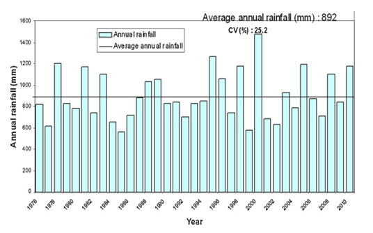
Fig. 8.1. Annual rainfall of India. (Source: http://www.sciencedirect.com/science/article/pii/S0378377412003058)

8.2.2 Mass Curve of Rainfall

The mass curve of rainfall is a plot of the accumulated precipitation against time, plotted in chronological order. Records of float type and weighing bucket type gauges are of this form. A typical mass curve of rainfall at a station during a storm is shown in Fig. 8.2

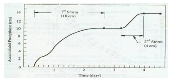
Fig. 8.2. Mass curve of Rainfall. (Source: http://theconstructor.org/water-resources/analysis-presentation-of-rainfall-data/4493/)

8.2.3 Double Mass Curve of Rainfall

The double mass curve technique, as illustrated in Fig. 8.3, is a reliable procedure for checking the consistency of a precipitation record. The technique compares long term annual or seasonal precipitation of a group of stations being evaluated. Some seasons of the year may have more inconsistencies than others. Therefore, seasonal analysis may provide better results than using total annual values. The accumulated annual or seasonal values for the comparison stations are plotted against the accumulated annual value for the evaluation station.

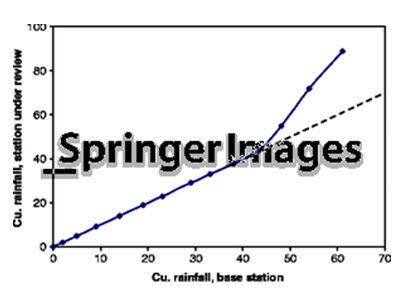
Fig. 8.3. Double Mass Curve of Rainfall. (Source: http://www.springerimages.com/Images/Environment/1-10.1007_978-1-4419-6335-2_3-4)

8.2.4 Hyetograph

Hyetograph is a plot of the intensity of rainfall against the time interval, as illustrated in Fig. 8.4. The Hyetograph is derived from the mass curve and is usually represented as a bar chart. It is a very convenient way of representing the characterstics of a storm and is particularly important in the development of design storms to predict extreme floods. The area under a hyetograph represents the total precipitation received in the period. The time interval used depends upon the purpose. In urban-drainage problems small durations are used while in flood-flow computations in larger catchments the intervals are of about 6 h.

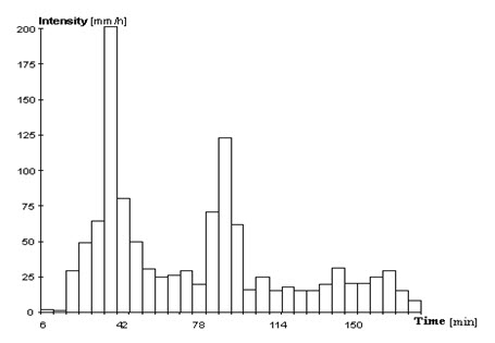
Fig. 8.4. Hyetograph. (Source: http://echo2.epfl.ch/VICAIRE/mod_1b/chapt_2/main.htm)

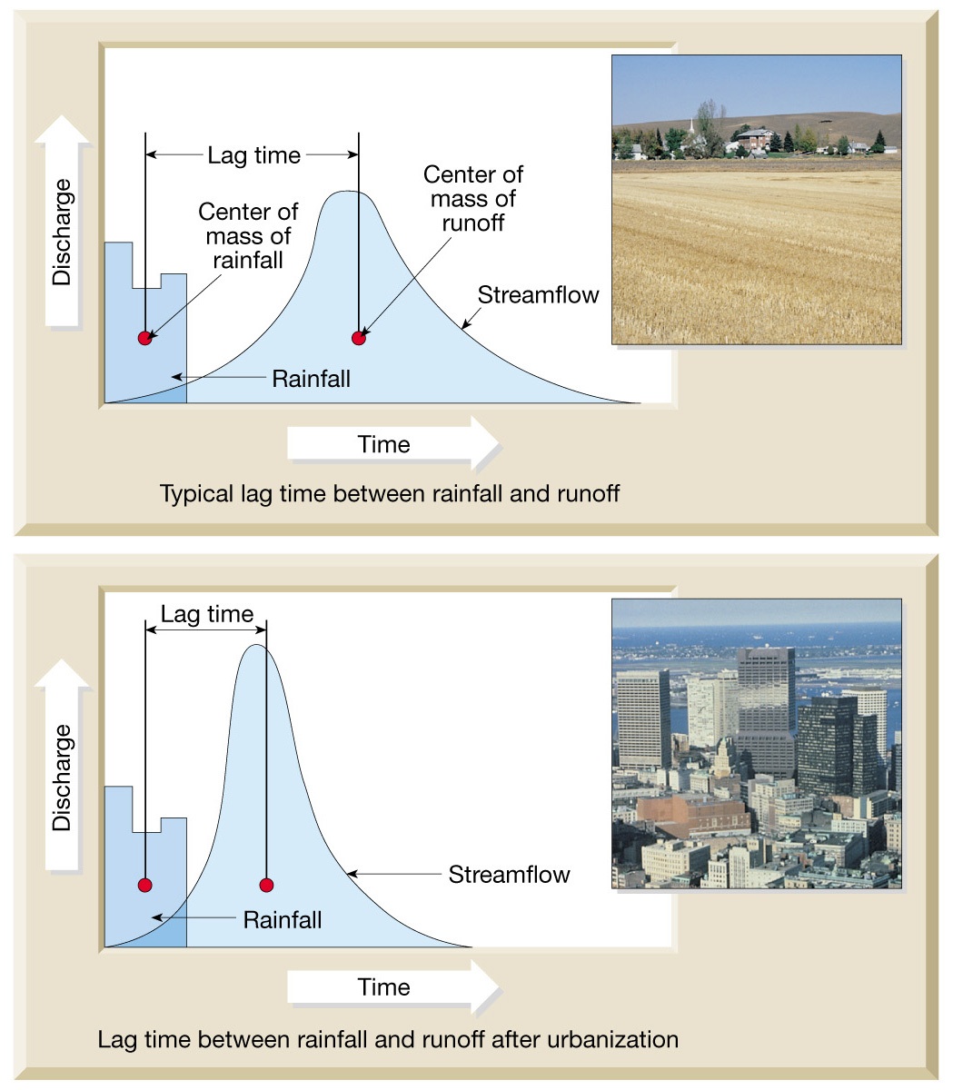
8.2.5 Hydrograph

The term "Hydrograph" stands for the graphical representation of the instantaneous rate of discharge of a stream plotted with respect to time, as illustrated in Fig. 8.5. This is as a result of the physiographic and hydrometerological effect of the watershed. Hydrographs are graphs which show river discharge over a given period of time and show the response of a drainage basin and its river to a period of rainfall. A storm hydrograph shows how a river's discharge responds following a period of heavy rainfall. On a hydrograph, the flood is shown as a peak above the base (normal) flow of the river.

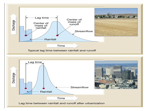
Fig. 8.5. Hydrograph. (Source: http://web.cortland.edu/barclayj/hydrograph.jpg)

8.2.6 Point Rainfall

The rainfall data measured at a place using a measuring device is known as point (or station) rainfall data. For small areas of less than 50 km², point rainfall may be taken as the average depth over the area. In large areas, there will be a network of rain-gauge stations. Depending upon the need, data can be listed as daily, weekly, monthly, seasonal or annual values for various periods. Graphically these data are represented as plots of magnitude Vs chronological time in the form of a bar diagram. Such a plot, however, is not convenient for subsequent uses. Fig. 8.6 shows the monthly precipitation.

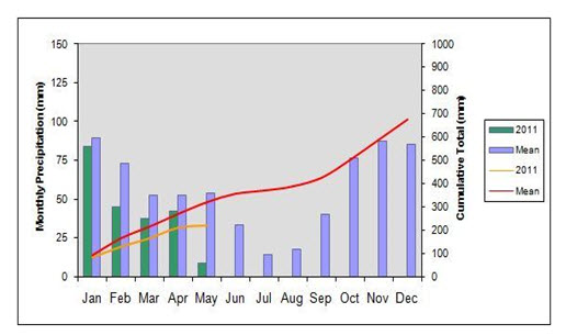
Fig. 8.6. Point Rainfall. (Source: http://malvedos.wordpress.com/2011/07/19/may-2011-douro-insider/)

v Mean Precipitation Over an Area: To convert the point rainfall values at various stations in to an average value over a catchment the following three methods are used: i) arithmetical-mean method (ii) Thiessen-polygon method (iii) Isohyetel method.

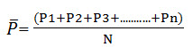
(i) Arithmetical-Mean Method:

When the rainfall measured at various stations in a catchment show little variation, the average precipitation over the catchment area is taken as the arithmetic mean of the station values. Thus if P₁,P₂,P₃....P_n are the rainfall values in a given period in N stations within a catchment, then the value of the mean precipitation  over the catchment by the arithmitic-mean method is

(ii) Thiessen Polygon Method

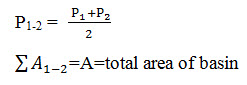
This method attempts to allow for non-uniform distribution of gauges by providing a weighting factor for each gauge, as illustrated in Fig. 8.7. The stations are plotted on a base map and are connected by straight lines. Perpendicular bisectors are drawn to the straight lines, joining adjacent stations to form polygons, known as Thiessen polygons. Each polygon area is assumed to receive uniform rainfall, as recorded by the raingauge station inside it, i.e., if P₁, P₂, P₃, .... are the rainfalls at the individual stations, and A₁, A₂, A₃, .... are the areas of the polygons surrounding these stations, (influence areas) respectively, the average depth of rainfall for the entire basin is given by:

where ΣA_i = A = total area of the basin.

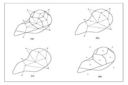
Fig. 8.7. Thiessen polygon method. (Source: http://daad.wb.tu-harburg.de/?id=279)

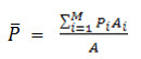
(iii) The Isohyetal Method

In this method, the point rainfalls are plotted on a suitable base map and the lines of equal rainfall (isohyets) are drawn giving consideration to orographic effects and storm morphology. The average rainfall between the successive isohyets taken as the average of the two isohyetal values are weighted with the area between the isohyets, added up and divided by the total area which gives the average depth of rainfall over the entire basin

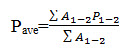
where A_1–2 = area between the two successive isohyets P₁ and P₂

• Intensity-Duration-Frequency Curve

The relationship between frequency, intensity and storm duration vary sufficiently from place to place and periodic revisions are desirable in each locality. The relationship between intensity-duration-frequency can be obtained from an analysis of rainfall records obtained at that location. The intensity of storm decreases with the increase in storm duration. Fig. 8.8 shows the intensity- duration curve over return period.

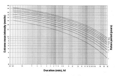
Fig. 8.8. Intensity-duration-frequency curve. (Source: http://civcal.media.hku.hk/yuenlong/introduction/_idfcurve.htm)

• Depth-Area-Duration Curve 

A depth-area-duration curve express graphically the relation between a progressively decreasing average depth of rainfall over a progressively increasing area from the centre of the storm outward to its edge for a given duration of rainfall. It can be constructed from any isohyetal map of rainfall for the given duration. Such a curve can be constructed for the duration (usually 6 h, 12 h, 18 h, 24 h, and 36 h) as shown in Fig. 8.9.

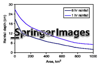
Fig.8.9. Depth-Area-duration curve. (Source: http://www.springerimages.com/Images/Environment/1-10.1007_978-1-4419-6335-2_3-1)

8.3 Simple Statistical Analysis

In the study of statistics we are basically concerned with the presentation and interpretation of chance outcomes that occur in a planned or scientific investigation. Hence, the statistician usually deals with either numerical data representing counts or measurements, or perhaps with categorical data that can be classified according to some criterion. We shall refer to any recording of information, whether it is numerical or categorical, as an observation. Statistical methods are those procedures that are used in the collection, presentation, analysis, and interpretation of data. These methods can be categorized as belonging to one of the two major areas called descriptive statistics and statistical inference.  

• Descriptive Statistics

Those methods concerned with collecting and describing a set of data so as to yield meaningful information. It provides information only about the collected data and in no way draws inferences or conclusions concerning a larger set of data.

• Statistical Inference

Those methods are concerned with the analysis of a subset of data leading to predictions or inferences about the entire set of data.

Fundamental

1. Hydrological Process

Hydrological environment consists of water inputs, environment response and the output. This union of three in one-input, response, output-is described as the basic parts of a hydrologic system, while each of these parts represents a hydrologic process. Natural hydrologic processes are never deterministic but are a combination of various deterministic and stochastic processes.

2. Deterministic Process

These are the processes of hydrology that are the results of physical, chemical and biological deterministic laws. For example, a rating curve of the stage discharge relationship of a river cross section with a fixed bed is a unique function and is thus a deterministic relation giving the same discharge for the same stage at all times.   

3. Stochastic Process

These are the processes of hydrology which are governed by the laws of chance such as precipitation, evaporation, and runoff. Stochastic models use random variables to represent processes with uncertainty and generate different results from one set of input data and parameter values when they run under “externally seen” identical conditions. A particular set of inputs will produce an output according to a statistical distribution. This allows some randomness or uncertainty in the possible outcome due to uncertainty in input variables, boundary conditions or model parameters. The application of flood frequency analysis in hydrologic design and operation of water resources systems are good examples of stochastic processes.

Mixed deterministic-stochastic models can also be created by introducing stochastic error models to the deterministic model. For example, stochastic rainfall could be used as an input to a deterministic rainfall-runoff model or a deterministic model may be used to represent a stochastic system. It is important to stress that the term chance, random, probabilistic and stochastic are considered synonyms. They all refer to the phenomena subject to the laws of chance.