Gulley & Ravine Control Structures 3(2+1)

Lesson 9 Analysis of Precipitation Data - II

9.2 Frequency of Point Rainfall

The rainfall occurring at a place is a random hydrologic process and the rainfall data at a place when arranged in chronological order constitute a time series. Thus, daily or weekly total rainfall arranged in a tabular fashion over a month or over a season constitutes the time series of daily or weekly rainfall. One of the commonly used data series is the annual series composed of annual values such as annual total rainfall. If extreme value of a specified event occurring in each year is listed, it also constitutes an annual series. Thus for example, one may list the maximum 24-h rainfall occurring in a year for the duration of 10 years. The probability of occurrence of an event in this series is studied by frequency analysis of this annual data series. The analysis of annual series, even though described with rainfall as a reference is equally applicable to any other random hydrological process.

The probability of occurrence of an event whose magnitude is equal to or in excess of a specified X is denoted by P. The recurrence interval (also known as return period) is defined as:  

 

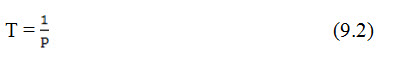
This represents the average interval between the occurrence of a rainfall of magnitude equal to or greater than X. Thus if it is stated that the return period of rainfall of 20 cm in 24 h is 10 years at a certain station A, it implies that an average rainfall magnitude equal to or greater than 20 cm in 24 h occurs at least once in 10 years.  In a long period of say 100 years, 10 such events can be expected. However, it does not mean that in every 10 years one such event is likely, i.e. periodicity is not implied.  The probability of a rainfall of 20 cm in 24 h occurring in any one year at station A is 1/T = 1/10 = 0.1.

If the probability of an event occurring is P, the probability of the event not occurring in a given year is q = (1-P). The binomial distribution can be used to find the probability of occurrence of the event r times in n successive years. Thus

P _{r ,n}  = ⁿ C _r P _r q ^{n – r} = [n ! /{(n -r )! r!} P _r q ^{n - r} ]                        (9.3)

Where, P _{r, n} = Probability of a random hydrologic event (rainfall) of given magnitude and exceedence probability of a random hydrologic event (rainfall) of given magnitude and exceedence probability P occurring r times in n successive years.

9.3 Stochastic Time Series

A time series may be defined as a set of observations arranged chronologically or it is a sequence of observations usually ordered in time but may also be ordered according to some other dimensions.

Time series can be conveniently be divided into two parts:

(1) Continuous Time Series

A continuous time series is a series in which the time variable is continuous. Conversely, even if the time variable itself may be continuous, the phenomenon being described may not necessarily be continuous for a given time, t. Unless analogous computations are carried out, continuous time series must be converted into a discrete form prior to analysis. One of the commonly used examples is the simulation of a chronological record of precipitation and runoff hydrograph.

(2) Discontinuous Time Series

A time series denoted by discrete number of time points, T_i; i = 1, 2....,N is defined as a discontinuous time series, even if the variable itself may be continuous. Thus, rainfall is a continuous variable but often for the convenience in analysis it may be discretised over small time durations.

Time series is used to generate data with the properties of the observed historical records to know the properties of a historical record. The time series is broken into individual components and then analyzed separately to understand the causal mechanism of the different components.

Classification of time series

The time series is classified into two types:

(a) Stationary

In this case, statistical parameters representing the series, such as the mean, standard deviation, etc. do not change from one segment of series to another. Consider for example a 20-year time series of annual maximum 1-day rainfall. This could be divided into two equal parts in several ways such as by making two time series of 10 years each or making two time series of nineteen years each (year 1-19 and year 2-20). Now if the two segments of the maximum 1-day rainfall data exhibit identical mean, identical standard deviation and so on; the 20-year time series will be called stationary.  However, this happens rarely with rainfall data of for that matter with most of the hydrologic data. The joint Probability distribution of a set of observations made at times t₁,t₂,.........t_N in a strictly stationary times series would be identical to that of another N observations made at times t₁ + k, t₂ + k,..........., t_N + k for all k. The statistical relationship between N observations at origin t is the same as the statistical relationship between N observations at origin t+k. These relationships are measured by correlation between any two time series observation separated by a "lag" of k time units.

(b) Nonstationary

In this, different segments of time series are dissimilar in one or more aspects, because of the effects of seasons and trends on the value of time series. Hydrological time series are invariably non stationary.

Method of Time-Series Analysis

A time series model for the observed data {x_t} is a specification of the joint distributions (or possibly only the means and covariances) of a sequence of random

variables {X_t} of which {x_t} is postulated to be a realization.

Models with Trend and Seasonality

For example, Yue et al. (2002a) investigated the interaction between a linear trend and a lag-one autoregressive [AR(1)] model using Monte Carlo simulation. Simulation analysis indicated that the existence of serial correlation alters the variance of the Mann-Kendall (MK) statistic estimate, and the presence of a trend alters the magnitude of serial correlation. Furthermore, it was found that the commonly used pre-whitening procedure for eliminating the effect of serial correlation on the MK test leads to inaccurate assessments of the significance of a trend. Therefore, it was suggested that firstly trend should be removed prior to ascertaining the magnitude of serial correlation. Both the suggested approach and the existing approach were employed to assess the significance of a trend in the serially correlated annual mean and annual minimum stream flow data of some pristine river basins in Ontario, Canada. It was concluded that the researchers might have incorrectly identified the possibility of significant trends by using the already existing approach.

A General Approach to Time Series Modeling

The following approach can be adopted for the analysis of a given set of observations:

(1) Plot the series and examine the main features of the graph, checking in particular:

Whether there is

(a) A trend,

(b) A seasonal component,

(c) Any apparent sharp changes in behavior,

(d) Any outlying observations.

(2) Identify, quantify and remove the deterministic trend and periodic components, thereby isolating the stationary stochastic component.

(3) Choose a model to fit the residuals, making use of various sample statistics including the sample autocorrelation function.

(4) Forecasting will be achieved by forecasting the residuals and then inverting the

Transformation described above to arrive at forecasts of the original series {X_t }.

9.4 Serial Correlation

A widely used measure of association between two variables  &  is the product moment correlation coefficient,

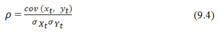
Where, the numerator is the covariance of    and ; where  and  may represent the rainfall events of the corresponding period in two consecutive years, and the denominator is the square root of the product of the variances of  and .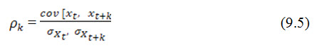

express the correlation which exists between all pairs of observations,  and , within the time series as a function of their spacing, k. The distance k is known as the lag between  and .  The numerator is referred to as the auto-covariance at lag k. The serial autocorrelation is thus used to account for the effect of serial dependence of series. If the value of time series X , say  at time unit t + k is dependent on the value of , then the correlation between the values of   and  may be taken as the measure of dependence.

The serial coefficient is therefore defined as the correlation coefficient between the members of the series that are k units apart.

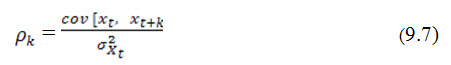
If the time series is stationary, then

then the equation becomes:

9.5 Markov Process  

Markov process describes only step by step dependence, called as first - order process, or shows lag-one serial correlation. A Markov process is defined in terms of discrete probabilities.

The probability relationship for a Markov process must provide for the conditional probabilities of the process moving from any state at period t to any subsequent  state at period t + 1. Thus

P = (X_{t+1= j}\X_{t = i})                                            (9.8)

Express the conditional probability of transitioning from state i at time t to state j at time (t + 1). Two conditions must be defined to describe the process completely.  One is the initial state, i.e. the value of the variable at the beginning, and the other is the complete matrix of transition probabilities.

A third and resultant property is a statement or matrix of steady-state probabilities which occur in all Markov processes after sufficient transitioning from state to state. The steady-state probabilities are independent of the initial state and transitioning probabilities.

9.6 White Noise Process

A process { (t)} is called a white noise if its values  (t_i) and  (t_j) are uncorrelated for every t_i and t_j  t_i. If the random variables (t_i) and (t_j) are not only uncorrelated but also independent, then { (t)} is called a strictly white noise process.

For a white noise process (t) with variance  the ACVF is given as:

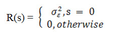
It will be assumed that the mean of a white noise process is identically zero, unless otherwise stated. White noise processes are important in time series analysis due to their simple structure.

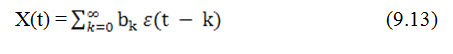
9.7 Moving Average Model MA(p)

By a moving average model of order p, denoted by MA(p), we mean a linear filter of the form

X(t) = ε (t) + b₁ ε (t - 1)  + ................+ b_p ε (t - p)               (9.9)

where, (t)  is a white noise process. In operator form, this can be written as

X(t) = P(B) ε (t)                                           (9.10)

where,

P(z) = 1 + b₁z + b₂z²+................ + b_pz^p                           (9.11)

and

BX(t) = X(t - 1),...................., BⁱX(t) = X(t - i)               (9.12)

MA(p) can be considered as an approximation of a more general form of X(t) in the form

by a finite parameter model. Then the spectral density function of X(t) is given by

9.8 Autoregressive Moving Average Model ARMA (q, p)

Autoregressive Moving Average (ARMA) models, also known as Box-Jenkins models, are typically used for analyzing and forecasting autocorrelated time series data. The ARMA model is based on two components, an autoregressive (AR) part and a moving average (MA) part, hence known as an ARMA(p,q) model where p is the order of  the autoregressive component based on prior observations of y or y values adjusted for systematic variations and q is the order of the white noise moving average component

A stochastic process X(t) is called an ARMA(q, p) model if it satisfies the difference equation 9.14:

X(t) + a₁X(t - 1) +..................+ a_qX(t - q) = ε (t)  + b₁ ε (t - 1)  + ........... + b_p ε (t - p)         (9.15)                                                                                 

In operator form this can be given as:

Q(z)X(t) = P(z) ε (t)                                      (9.16)

where Q(z) =  1 + a₁z + a₂z² + .............................+ a_qz^q

 and   P(z)  =   1 + b₁z + b₂z² + .................. + b_pz^p

The model possesses a stationary solution only if Q(z) has no zeros inside or on the unit circle.

An ARMA (q; p) model is characterized by a rational transfer function of the form:

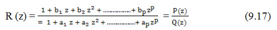
In engineering literature, MA models are known as all zero models while AR models are known as all-pole models. ARMA models are referred to as pole-zero models.

An ARMA (1;1) process has the general structure:

X(t) = a X (t - 1) + b  ε (t - 1) + ε (t)                        (9.18)

9.9 Autoregressive Integrated Moving Average Model ARIMA (q, r, p)

Box and Jenkins (1970) considered a slightly more general model called ARIMA (q, r, p) in which case Q (B) contains a factor of the form (1 - B)^r. Then the transfer function R (z) has a r^th order pole at z = 1. Consequently X (t) turns out to be a non stationary process. However, its r^th difference  X (t) would be stationary.

When r = 0, we get the ARMA (q, p) model. The ARIMA (q, r, p) model can be given in the operator form as:

Ø (B)(1- B)^r X(t) = θ (B) (t)                                 (9.19)

This Eqn. 9.17 can be rewritten as:

Ø (B) Y(t) = θ (B) ε (t), Y(t) = Δ^r X(t), Δ = 1 – B             (9.20)

Then the reduced process Y(t) Eq. 9.20 will be a stationary ARMA model.