Gulley & Ravine Control Structures 3(2+1)

Lesson 11 Computation of Runoff

11.2 Rational Method

The Rational Method is most effective in urban areas with drainage areas of less than 80 hectare.  The method is typically used to determine the size of storm sewers, channels, and other drainage structures.  This method is not recommended for routing storm water through a basin or for developing a runoff hydrograph. However, for the sake of simplicity, the Rational Method is used to determine the size of the detention basin required for construction site.  

The rational method is based on a simple formula that relates runoff-producing potential of the watershed, the average intensity of rainfall for a particular length of time (the time of concentration), and the watershed drainage area. The formula is

Q = 0.28 * C * I * A

Where Q = design discharge (m³/s), C = runoff coefficient (dimensionless), I = design rainfall intensity (mm/h), and A = watershed drainage area (km²).

Modified Rational Method

The Modified Rational Method (as shown in Fig. 11.1) provides a way to calculate the hydrograph from a catchment based on rational method, C values and the peak intensity. There is no "loss method" associated with the modified rational method. The underlying assumption is that the peak intensity is maintained for long enough duration to reach peak flow at the outlet of the catchment. This results in a trapezoidal hydrograph as shown in Fig. 11.1.

In the modified version of the rational formula, a storage coefficient, C_s, is included. In the original formula the recession time was assumed to be equal to the time of rise. The modified rational method is then described by the formula:

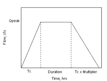
Fig. 11.1. Trapezoidal hydrograph. (Source: http://docs.bentley.com/en/HMCivilStorm/Help-15-120.html)

Q_p = 0.28*C_s*C*I*A

Where C_s is storage coefficient; C, A, I, are same as that of Rational Method.

In the modified version of the Rational Formula, a storage coefficient (C_s) is included to account for a recession time larger than the time the hydrograph takes to rise.

11.3 Kinematic Wave Technique

The kinematic wave technique is a simplified version of the dynamic wave technique. The full dynamic wave technique takes into account the entire spectrum of the physical processes, which simulate hydrologic flow along a stream channel. The kinematic wave simplifies these processes by assuming various physical processes as negligible. Dynamic wave models are based on one-dimensional gradually varied unsteady open channel flow. The dynamic wave consists of two partial differential equations (continuity and momentum), otherwise referred to as the Saint-Venant equations. The Saint-Venant equations take into account the physical laws, which govern both conservation of mass (continuity) and conservation of momentum (dynamic). These physical factors consist of local acceleration, convective acceleration, hydrostatic pressure forces, gravitational forces, and frictional forces.

Kinematic wave models are based on the continuity equation and a simplified form of the momentum equation used for the full dynamic wave. The physical factors which govern the kinematic wave are gravitational forces and frictional forces.

11.3.1 Continuity Equation

The continuity equation applies to both dynamic waves and kinematic waves. The equation is based on the principle of the conservation of mass and is written as:

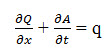
Where, Q is the discharge (m³ s^-1), A is the cross-sectional area (m²), q is the lateral inflow per unit length (m³ m^-1), x is the space coordinates (m), and t is the time (seconds).

11.3.2 (a) Momentum Equation (Dynamic Wave Form)

The momentum equation applies to the full dynamic wave. The equation is based on Newton’s second law of motion and is written as:

Where, y is the flow depth, V is the mean velocity, g is the gravitational acceleration, S_o is the bed slope, and S_f is the friction slope.

11.3.2 (b) Momentum Equation (Kinematic Wave Form)

The simplified version of the full dynamic wave equation applies to kinematic waves. This equation is

S_f = S_o

Where, S_f is the friction slope and S_o is the bed slope (gravity).

11.4 Neural Network for Runoff Modeling

The Artificial Neural Network (ANN) is an information processing system composed of many nonlinear and densely interconnected processing elements or neurons, which are arranged in groups called layers. The basic structure of an ANN usually consists of three layers: the input layer, where the data are introduced to the network; the hidden layer or layers, where data are processed; and the output layer, where the results of given input are produced. The inter-connection between neurons is accomplished by using known inputs and outputs, and presenting these to the ANN in some ordered manner; this process is called training. The strength of these interconnections is adjusted using an error convergence technique so that a desired output will be produced for a known pattern. The main advantage of the ANN approach over traditional methods is that it does not require information about the complex nature of the underlying process under consideration to be explicitly described in mathematical form. The merits and shortcomings of this methodology have been discussed in a recent review by the ASCE task committee on application of ANNs in hydrology (ASCE, 2000a,b). They have indicated that rainfall-runoff modelling has received maximum attention by ANN modellers. In a preliminary study, Halff et al. (1993) designed a three-layer feed-forward ANN using the rainfall hyetographs as input and hydrograph as output. This study opened up several possibilities for rainfall-runoff modeling.

The feed-forward multilayer perceptron (MLP) is the most commonly used ANN in hydrological applications. The structure of a three-layer MLP is shown in Fig. 11.2 and its further elaboration in Fig. 11.3.  The number of neurons in the input and output layers are defined based on the number of input and output variables of the system under investigation, respectively. However, the number of neurons in the hidden layer(s), in a study, e.g. a single hidden layer with six neurons, is usually defined via a trial-and-error procedure. As seen from the figure, the neurons of each layer are connected to the neurons of the next layer through weights. In order to obtain optimal values of these connection weights, ANNs must be trained. In some cases, a back-propagation algorithm for training the network, in which the inputs are presented to the network and the outputs obtained from the network are compared with the real output values (target values) of the system under investigation in order to compute error and then the computed error is back-propagated through the network and the connection weights are updated. This procedure, called training procedure, continues until an acceptable level of convergence is reached. In many studies, in order to avoid instability, the neural network is trained a number of times, and by averaging the output from all, a final output is obtained.

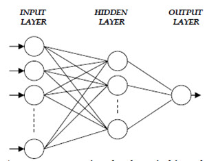
Fig. 11.2. The structure of a 3-layer MLP. (Source: http://research.guilan.ac.ir/cjes/.papers/958.pdf)

Fig. 11.3. The structure of a 3-layer MLP. (Source: http://research.guilan.ac.ir/cjes/.papers/958.pdf)

11.5  Storm Water Management Model (SWMM)

The EPA Storm Water Management Model (SWMM) is a dynamic rainfall-runoff simulation model used for single event or for long-term (continuous) simulation of runoff quantity and quality from primarily urban areas. The runoff component of SWMM operates on a collection of sub-catchment areas on which rain falls and runoff is generated. The routing portion of SWMM transports this runoff through a conveyance sys­tem of pipes, channels, storage/treatment devices, pumps, and regulators. SWMM tracks the quantity and quality of runoff generated within each sub-catchment, and the flow rate, flow depth, and quality of water in each pipe and channel during a simulation period comprised of multiple time steps.

The model is organized in the form of “blocks”. There are four computational blocks and six service blocks in the model (as shown in Fig. 11.4). However, the model is usually run using only the executive block and one or two computational blocks. The runoff and extended transport computational blocks and the executive and graph service blocks are normally used in various studies. The runoff block accepts rainfall and calculates infiltration, surface detention, and overland and channel flow. Rainfall depths from actual storms are used to make the estimates. The SWMM model has two options for calculating infiltration. The first one uses the Green-Ampt equation. The second one uses an integrated form of Horton's equation. Both the Green-Ampt equation and Horton's equation are used in separate simulations. Except for the urban watersheds, infiltration is also routed through subsurface pathways. Subsurface routing is calculated in the runoff block.

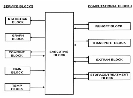
Fig. 11.4. SWMM, the Storm Water Management Model, program configuration. (Source: http://rpitt.eng.ua.edu/Class/Computerapplications/Module9/Module9.htm)

11.6 The TOPMODEL

It is a rainfall-runoff model that bases its distributed predictions on an analysis of catchment topography. The model predicts saturation excess and infiltration excess surface runoff and subsurface storm flow. Since the first article was published on the model in 1979 there have been many different versions. The idea has always been that the model should be simple enough to be modified by the user so that the predictions conform as far as possible to the user's perceptions of how a catchment behaves. The distributed outputs from the model (as shown in Fig. 11.5) help in such assessments.

The TOPMODEL framework has two components: (1) the storage component, which is represented by three reservoirs and (2) the routing component, which is derived from a distance-area function and two velocities parameters. Its main parameter is the topographic index derived from a digital elevation model. This index represents the propensity of a cell or region to become saturated. The TOPMODEL is considered as a semi-distributed model, as it uses distributed topographic information to determine the topographic index and to distribute saturation deficits throughout the basin, as well. However, its main limitation is the impossibility to use distributed input data, such as rainfall and evapotranspiration

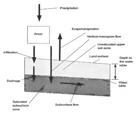
Fig. 11.5. Water fluxes when rainfall or snowmelt occurs on an unsaturated location in the watershed. (Source: http://pubs.usgs.gov/wri/1993/4124/report.pdf)

11.7 Flood Estimation for Gauged Watershed

For a small watershed, the design flood hydrograph can be synthesized from available storm records using rainfall-runoff models, but in case of large watersheds, which provide some hydrological data, a calculated risk can be taken in designing hydraulic structures for a flood lesser than the most severe flood.

A method of dealing with the runoff directly is called the flood frequency method. The method does not provide a hydrograph shape but gives only a peak discharge of known frequency. Frequency studies interpret a past record of events to predict the future probabilities of occurrence. If the runoff data are of sufficient length and reliability, they can yield satisfactory estimates. In most cases, records extend to short length of time and contain relatively few events. Such records when analyzed are likely to lead to inconsistent results as they are not representative of long term trend.

The value of the annual maximum flood from a given catchment area for large number of successive years constitutes a hydrological data series called the annual series. The data are then arranged in descending order of magnitude and the probability P of each event being equal to or exceeding (plotting position) is calculated by the plotting position formula. If the probability of an event occurring is P, the probability of the event not occurring in a given year is q = (1-P). The binomial distribution can be used to find the probability of occurrence of the event r times in n successive years. Thus

P _{r ,n}  = ⁿ C _r P _r q ^{n - r}= [n ! /{(n -r )! r!} P _r q ^{n - r} ]

Where, q = 1-P 

Two distributions which are widely employed in recent years are: (i) the logarithmic normal and (ii) the extreme value. The methods of analysis based on these distributions can be grouped as: (i) curve fitting methods, graphical or mathematical and (2) methods using Frequency factors comprising:  (a) the Gumbel method (b) the lognormal method and (c) other methods such as Foster III, Foster I and Hazen methods.

The curve fitting methods based on frequency factor for hydrologic frequency analysis:

x =   + Ks

Where, x = flood magnitude of given return period T,  = mean of recorded floods, s = standard deviation of recorded floods, K = frequency factor

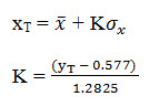
(a) Gumbel's Method

Gumbel's distribution is one of the widely used probability distribution functions for extreme values in hydrologic and meteorologic studies for prediction of flood peaks, maximum rainfall, maximum wind speed etc. Gumbel defined a flood as the largest of the 365 daily flows and the annual series of flood flow that constitutes a series of largest value of flows. The probability of occurrence of an event equal to or larger than a value of

In which, y is a dimensionless variable given by

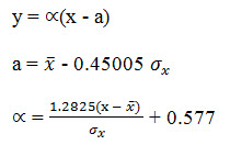
Where,   = mean and  = standard deviation of the variate X. In practices it is the value of X for a given P that is required, y_p = - ln [- ln (1 - P)]

Noting that the return period T = 1/P and designating

 

Now rearranging, the value of the variate X with a return period T is

Confidence Limit

Since the value of the variate for a given return period, x_T determined by Gumbel's method can have errors due to the limited sample data used; an estimate of the confidence limits of the estimate is desirable. The confidence interval indicates the limit of the calculated value between which the true value can be said to lie with a specific probability based on sampling errors only.

For a confidence probability c, the confidence interval of the variate, x_T is bounded by values x₁ and x₂ given by

x_1/2 = x_T  ± ƒ (c) S_e

Where, ƒ (c) = function of the confidence probability c determined by using the table of normal variates.

(b) Log-Pearson Type III Distribution

The statistical distribution most commonly used in hydrology in the United States is the log-Pearson Type III (LP3) because it was recommended by the U.S. Water Resources Council in Bulletin 17B (Interagency Advisory Committee on Water Data, 1982). It is widely accepted because it is easy to apply when the parameters are estimated using the method of moments and it usually provides a good fit to measured data.

This method is applied in the following steps:

1. Transformation of the n annual flood magnitudes, Xi, to their logarithmic values, Yi (Yi = log Xi for i=1, 2, .....n).

2. Computation of the mean logarithm, .

3. Computation of the standard deviation of the logarithms, SY.

4. Computation of the coefficient of skewness, Cs.

 

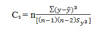
5.  Computation of

Where, K_T is obtained is obtain from table 11.1.

6. Computation of XT = antilog YT.

This method has as a special case the lognormal distribution when CS = 0.

Table 11.3 Skew coefficient for Log Pearson III

(Source: http://www.nzdl.org/gsdlmod?e=d-00000-00---off-0hdl--00-0----0-10-0---0---0direct-10---4-------0-1l--11-en-50---20-home---00-0-1-00-0-0-11-1-0utfZz-8-10&a=d&cl=CL1.8&d=HASH3b4d99e5f9716ab628b9b2.11.fc)

(c) Log- Normal Method

If the random variable Y = log X is normally distributed, then X is said to be log-normally distributed. Chow(1954) reasoned that this distribution is applicable to hydrologic variables formed as the product of other variables since if X = X₁  X₂  X₃ X₄ ....X_n, then Y , which tends to the normal distribution for large n provided that the Xi are independent and identically distributed.

For the lognormal distribution, the frequency factor is given by chow (1964) as

K_T = [exp (σ_y K_y  - σ²_y/2)-1]/[exp(σ²_y )-1]^1/2

Where, Y = ln X and K_Y = (YT - µY)/σ_y

The lognormal distribution has the advantages over the normal distribution that it is bounded (X > 0) and that the log transformation tends to reduce the positive skewness commonly found in hydrologic data, since taking logarithms reduces large number proportionately more than it does for small numbers. Some limitations of the lognormal distribution are that it has only two parameters and that it requires the logarithms of the data to be symmetric about their mean.

• Regional Flood Frequency Analysis

This technique of frequency analysis to develop a frequency curve at a gauging station on a stream has been dealt with at length in the preceding section. Extension of the result of the frequency analysis of station data to an area requires regional analysis. The regional flood frequency analysis aims at utilizing available records of stream in the topographically similar region on either side of the stream in question so as to reduce sampling errors. The analysis consists of two major parts. The first is the development of the basic dimensionless frequency curve representing the ratio of the flood of any frequency to the mean annual flood. The second part is the development of relation between topographic characteristics of the drainage area and mean annual flood to enable the mean annual flood to be predicted at any point within the region. The combination of the mean annual flood with the basic frequency curve, which is in terms of the mean annual flood, provides a frequency for any location.

• Procedure

The following steps can be followed for regions where the Gumbel method produces a flood frequency reasonably accurate at individual stations. The stepwise procedure is given below:

1. All stations in the region with 10 or more year’s record are selected.

2. A frequency curve covering the range up to the 100- years flood is obtained by the Gumbel method for each of the individual stations and confidence limits are constructed with 95% reliability on each of these frequency curves.

3. A homogeneity test on the 10-year flood is performed as:

(a) The ratio of the 10-year flood to the mean annual flood is determined from the frequency curve of each station. These ratios are averaged to obtain the mean 10-year ratio for the year.

(b) The return period corresponding to the mean annual flood times the mean 10-year ratio is determined from the frequency curve of each station and plotted against the number of years of record for that station on a test graph. If the points for all of the stations lie between the 95% confidence limits, then they are considered homogenous.

The 95% confidence band, the spread to be expected for the chance variation on the test graph, the upper and lower limits of a 10-year flood for each station are computed corresponding to the 95% confidence band. The test is performed on a 10-year flood as it is the longest recurrence interval for which most records will give dependable estimates.

4. A set of flood ratios (ratio of flood to mean annual flood) is computed for each of the stations satisfying the homogeneity test for different return periods with the help of station frequency curves.

5. For each selected return period, the median of the ratio from all the stations is computed. The resulting medians values give the regional curve. These are plotted on an extreme value probability paper and the best fit line is drawn through them. This line is the required regional frequency curve.

Since the number of stations in the region is generally less than 10 for want of data in developing countries, the mean is a more stable parameter than the median. The CWC recommends the use of the mean instead of the median in the above analysis.

6. To compute confidence band limits for the regional curve, the width of the confidence band at arbitrarily selected return periods is read from each of the individual curves. The widths are then divided by the respective mean annual floods to produce a set of ratios which may be called errors in the individual curves. The errors are combined by computing the root of the sum of their squares and then dividing by the number of stations. The resulting ratio is taken as the error in the regional error estimate, i.e. the width of the confidence band for the regional curve at the selected return period. The procedure is repeated with another return period.

• Application to Ungagged Basin

Regional frequency curves have their most useful application in estimating the flood potential of an ungauged basin, since such curves show the ratio of flood to the mean annual flood for the ungauged basin. The mean annual flood is dependent upon many variables, the most important and commonly available being the drainage area. A correlation is usually therefore established graphically by plotting mean annual flood against respective drainage areas of all gauged stations in the region on logarithmic paper and the relation is used to obtain the mean annual flood for the region having the ungauged area. The flood of any given frequency for the ungauged area is then obtained by determining the corresponding flood ratio from the regional-frequency curve for the region of which the ungauged basin is a part and multiplying it by the estimated mean annual flood of the ungauged basin.