Irrigation Engineering 4(3+1)

LESSON 38 Design of Sprinkler Irrigation System-II

38.1 Hydraulic Design of Pipe Network

As stated in previous lesson, the pipe network in the sprinkler irrigation system consists of the lateral, sub main and main pipeline. The sprinkle nozzles are mounted on the laterals; laterals are connected to the sub main and sub main to the main. Main pipe line takes water from the source through the pump. It is desired to design the pipe network appropriately for uniform water application and economical system cost. As the sprinkler system requires pressure to operate, both uniformity water application and system economy are affected by the frictional head loss through the pipes. Large variation in friction head loss in the lateral or sub main reduces the uniformity in water application on the other hand too small variation results in high uniformity, which requires larger pipe size makes system more expensive. Hence it requires optimal combination of hydraulic and economic consideration.

 

There are several formulae available in the literature for estimating frictional head loss through sprinkler pipes.

 

However the Hazen-Williams equation is commonly adopted and given by

                                       (38.1)

 

Where,

H_f (100) = a friction loss per 100 m (100 ft) of pipe, m/100 m. 

C = a friction coefficient which is a function of pipe material characteristics;

Q = the flow of water in the line L s^-1 (ft³ s^-1) (gal min^-1);

D = the inside pipe diameter, mm (ft) (in.);

K = a constant which is 1.22 × 10¹² for metric units, 473 for Q in ft³ s^-1 and D IN ft, and 10.46 for Q in gal min^-1 and D in inch: the value C increases as the pipe increases. As the number of couplers decreases, the value C increases. Pipe materials with smoother inside wall will have a higher C value. Table 38.1 provides the values of C for different pipe materials.

 

Table 38.1. Typical values of C for use in Hazen-Williams equation

Sl. No.	Pipe material	C
1	Plastic	150
2	Epoxy-coated steel	145
3	Cement asbestos	140
4	Galvanized steel	135
5	Aluminum (with coupler every 9.0 m)	130
6	Steel (new)	130
7	Steel (15 years old) or concrete	100

(Source: Keller and Bliesner, 1990)

 

Flow Velocity in Pipe: Normally flow velocities in pipes should not exceed 3m s^-1 (10 ft s^-1). For permanent systems with polyvinyl chloride (PVC) plastic pipe, and asbestos cement (AC) pipe used for water supply, water flow velocity should not exceed 2.25 m s^-1 and most manufactures caution against using water flow velocity in excess of 1.6 m s^-1.

Allowable Head Loss in Sprinkler Pipe: Pressure loss occurs due to friction and joints. This should not exceed practical value. Normally it should be between 15 and 20 per cent of the total head. The recommended practice to design the sprinkler lateral is not to exceed the pressure variation more than 20% of the higher pressure. The difference in elevation head is considered while determining the variation in pressure. This may be paying of laterals in upward slope or down slope. While the lateral is laid on up slope direction, the less pressure is available at the nozzle while lateral laid on down slope direction, the additional pressure is available at the sprinkler nozzle due to gain in energy.

Pipe with Multi Outlet: When there are no outlets along the length of the lateral or sub main (usually called as closed pipe line or blind pipe), the head loss due to friction can be computed by Hazen-William formula (Equation 38.1). However, in sprinkler lateral or sub main, outlets along the length of the pipe are given as sprinkler heads or sprinkler laterals as the case may be. Flow of water through the closed or blind pipe of a given diameter causes more frictional head loss compared to that of a pipe with number of outlets along the length of the pipe which is due to the fact that the flow rate decreases with every passing outlet. To accurately compute friction loss in the lateral with multi outlet, start at the last outlet on the pipe line and work back to the head of the pipeline, computing the friction head loss between each outlet for the flow rate between two outlets. Table 38.2 is a ready reckoner table for estimation of head loss due to friction from aluminum pipe. Christainsen (1942) has simplified the procedure for choosing size of pipe for a given discharge and friction loss (Table 38.2). In case of multiple outlets the frictional head loss through the blind pipe is computed for the given flow rate and then multiply with reduction factor (F) due to reducing flow rate. The reduction factor depends on the number of equally spaced outlets on the lateral.

 

Table: 38.2 Friction head loss in irrigation pipes.

Friction head loss in meters per 100 meters in lateral line of portable aluminum pipe with coupling (Based on Scobey’s formula and 9 meters pipe length) 

Flow litres/sec	Diameter of pipe
	5.0 cm Ks 0.34	7.5 cm Ks 0.33	10.0 cm Ks 0.32	12.5 cm Ks 0.32	15.0 cm Ks 0.32
1.26	0.32
1.89	2.53
2.52	4.49	0.565	0.130
3.15	6.85	0.858	0.198
3.79	9.67	1.21	0.280
4.42	12.9	1.63	0.376	0.122
5.05	16.7	2.10	0.484	0.157
5.68	20.8	2.63	0.605	0.196
6.31	25.4	3.20	0.738	0.240	0.099
7.57		4.54	1.04	0.339	0.140
8.83		6.09	1.40	0.454	0.188
10.10		7.85	1.80	0.590	0.242
11.36		9.82	2.26	0.733	0.302
12.62		12.0	2.76	0.896	0.370
13.88		14.4	3.30	1.07	0.443
15.14		16.9	3.90	1.26	0.522
16.41		19.7	4.54	1.47	0.608
17.67		22.8	5.22	1.70	0.700
18.93		25.9	5.96	1.93	0.798
20.19		29.3	6.74	2.18	0.904
21.45		32.8	7.56	2.45	1.02
22.72		36.6	8.40	2.74	1.13
23.98		40.6	9.36	3.03	1.26
25.24		44.7	10.3	3.34	1.38
26.50			11.3	3.66	1.51
27.76			12.3	4.00	1.66
29.03			13.4	4.35	1.80
30.29			14.6	4.72	1.95
31.55			15.8	5.10	2.12
34.70			18.9	6.12	2.52
37.86			22.2	7.22	2.98
41.01			25.9	8.40	3.46
44.17			29.8	9.68	3.99
47.32			33.8	11.0	4.54
50.48				12.5	5.15
53.63				14.0	5.78
56.79				15.6	6.44
59.94				17.3	7.14
63.10				19.0	7.86

(Source:  Michael, 2010)

 

Assuming first sprinkler is at the same as other sprinklers located on the lateral, The F can be computed using following expression (Christiansen, 1942).

                 F =                                                (38.2)

 

where

F = reduction factor

N = number of outlets

m = exponent used in the head loss equation (In Hazen-William’s equation the m = 1.852 and for Darcy’s Weisbach equation m=2)

 

For N>10, the last term in equation 38.2can be omitted.

 

Jensen and Fratini (1957) modified the above expression for F to account for the first sprinkler being located one-half the sprinkler spacing from the supply line. They assumed that no water flows past the last sprinkler. The modified expression (Equation 38.3) indicates that the F factor is more than 5 percent larger for N<20.

               (38.3)

 

Estimates of F values are easy to obtain using Equation (38.2), but these estimates become much more tedious when using equation (38.3) for large values of N. To simplify their use, F values for m = 1.90 are presented in Table 38.3.

38.1.1 Design of Sprinkler Laterals

As stated earlier in design of sprinkler laterals the pressure variation should not exceed more than 20% of the higher pressure. The design capacity for sprinklers on a lateral is based on the average operating pressure.

Table 38.3. Reduction factor ‘F’ for friction loss in aluminum pipe with

No. of sprinklers on lateral	1st sprinkler is one sprinkler interval from main	1st sprinkler is 1/2 sprinkler interval from main	No. of sprinklers on lateral	1st  sprinkler is one sprinkler interval from main	1st sprinkler is1/2 sprinkler interval from main
1	1.000	1.000	16	0.365	0.345
2	0.625	0.500	17	0363	0.344
3	0.518	0.422	18	0.361	0.343
4	0.469	0393	19	0.360	0.343
5	0.440	0.378	20	0.359	0.342
6	0.421	0.369	22	0.357	0.341
7	0.408	0.363	24	0.355	0.341
8	0398	0.358	26	0.353	0.340
9	0.391	0.355	28	0.351	0.340
10	0.385	0.353	30	0.350	0.339
11	0.380	0.351	35	0.347	0.338
12	0.376	0.349	40	0.345	0.338
13	0.373	0.348	50	0.343	0.337
14	0.370	0.347	100	0.338	0.337
15	0.367	0.346	>100	0.335	0.335

multiple outlets

(Source:  Michael, 2010)

 

Where, the friction loss, H_f in the laterals is within 20% of the average pressure.

The average pressure head, can be expressed approximately by

                                       (38.4)

where,  = pressure at the sprinkler on the farthest end.

If the lateral is on nearly level land or on the contour, the head at the main is given

         H_n = H_o + H_f                                                                                 (38.5)

 

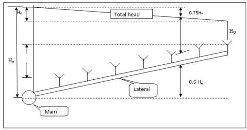
Fig. 38.1. Pressure profile in a lateral laid uphill. (Source: Michael, 2010)

 Solving Equation (38.4) in terms of H_o and substituting in Equation 38.5it becomes

                                 (38.6)

 

where,

H_a = Average pressure

H_f = Head loss due to friction in lateral pipe       

H_n = Pressure required at the main to operate, m

H_e = Maximum difference in elevation between the first and last sprinkler on a lateral pipe, m

H_r = the riser height, m

 

The term  is positive if lateral is laid up slope and negative, if lateral is laid down slope

 

38.1.2 Design of Main Pipe

As stated earlier the sub main pipe supplies the water to sprinkler lateral and main supplies water to the sub main. If more numbers of sub mains are operated simultaneously at same time (a case for the large field) the procedure described for the design of the lateral may be used. However, when a single sub main is operated, the size of sub main and main pipe line is selected such that the annual operating cost and initial cost of the sub main line and mainline should be low.

Normally friction loss of 3 m for small sprinkler system and 12 m for large sprinkler systems are used in design of main pipe line.

 

38.2 Pumps and Power Units

The suitable size of pump is selected considering the maximum total head against which the pump expected to operate and deliver the required discharge. This is be determined by

                                   (38.7)

 

where,

H_t = total design head against which the pump is working, m

H_n = maximum head required at the main to operate the sprinklers on the lateral at the required average pressure, including the riser height, m

H_m = maximum friction loss in the main and in the suction line, m

H_J = elevation difference between the pump and the junction of the lateral and the main, m, and

H_s= elevation difference between the pump and the source of water after drawdown, m

 The discharge required to be delivered by pump is determined by multiplying the number of sprinklers that are operated at any given instant of time by the discharge of each sprinkler. Once the head and discharge of the pumps are known, the pump may be selected from rating curves or tables provided by the manufacture.

 The horse power requirement of pump is given by

 

    h_p = Q_t × H_t / 75 × n_P                               (38.8)

 

Q_t = total discharge, L s^-1,

H_t = total head, m

n_p = efficiency of pump(fraction)

 

Example 37.1:

Design a sprinkler irrigation system to irrigate 5 ha Wheat crop.

Assume

Soil type = silt loam, Infiltration rate at field capacity = 1.25 cm h^-1, Water holding capacity = 15 cm m^-1, Root zone depth = 1.5 m, Daily consumptive use rate           = 6 mm day^-1, Sprinkler type = Rotating head.

 

This example is adopted from Tiwari (2009).

 

Solution:

Step I

Given infiltration capacity =1.25 cm h^-1

Hence maximum water application rate = 1.25 cm/h

 

Step II

Total water holding capacity of the soil root zone = 15 x 1.5 = 22.5 cm

Let the water be applied at 50% depletion, hence the depth of water to be

applied = 0.50 x 22.5 = 11.25 cm

Let the water application efficiency be 90 per cent

Depth of water to be supplied = 11.25 / 0.9 = 12.5 cm

 

Step III

For daily consumptive use rate of 0.60 cm

Irrigation interval = 11.25 / 0.6 = 19 days

In period of 19 days, 12.5 cm of water is to be applied on an area of 5 ha. Hence assuming 10 hrs. of pumping per day, the sprinkler system capacity would be

 Step IV

Let the spacing of lateral (Sm) = 18 m,

Spacing of Sprinklers in lateral (Sl) = 12 m  

This selection is based on using following consideration:

Operating pressure of nozzle         = 2.5 kg cm^-2

Maximum application rate             = 1.25 cm h^-1

 Referring sprinkler manufacturer’s M/S NOCIL, Akola catalogue (Table 38.4), the nozzle specifications with this operating pressure and application rate is:

Nozzle size                : 5.5563 x 3.175 mm

Operating pressure    : 2.47 kg/cm² and

Application rate         : 1.10 cm hr^-1 (which is less than the maximum allowable application rate of 1.25 cm h^-1)

Diameter of coverage  : 29.99 ≈ 30.0 m

Discharge of the nozzle : 0.637 L s^-1 = 0.637 x 10^-3 m³s^-1

 

Step V

Total no. of sprinkler required =  = 14.12 ≈ 14 sprinklers

Considering two sprinkler laterals, therefore 7 sprinklers on each lateral.

 

Step VI

Using Table 38.3, the sprinklers spaced at 12 m intervals on each lateral. The lateral lines will be at 18 m spacing.

 

Step VII

Total length of each lateral = 12 x 7 = 84

Operating pressure = 2.47 kg cm^-2

 

Total allowable pressure variation in the pressure head is 20%, hence maximum allowable pressure variation in pressure = 0.2 x 2.47 = 0.494 kg/cm² = 4.94 m

Assume pressure variation due to elevation = 2 m

Permissible head loss due to friction   = 4.94 – 2 = 2.94 m

Total flow through the lateral = 7 x 0.637 x 10^-3 = 4.459 x 10^-3 m³s^-1

Reduction factor (F) =  = 0.333 + 0.071 + 0.0034 = 0.407

 

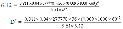
Head loss due to friction = using Darcy’s weisbach equation and reduction factor.

H_f =

or  2.94 =

 

Hence diameter of lateral = 63 mm

Assume height of riser pipe =1 m

The head required to operate the lateral lines (H_m) = 24.7 + 2.94 + 2 + 1 = 30.6 m

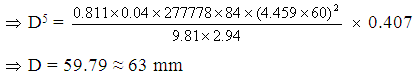
Frictional head loss in main pipe line (H_f) = 30.6  0.2 = 6.12 m

 

Calculating in the same way as done in case of lateral

 

or

D = 69.10 ≈ 75 mm

Total design head (H) = H_m+ H_f +H_j +H_s

 

Where,

H_j = Difference in highest junction point of the lateral and main from pump  

level = 0.5 m (assume)

H_s = Suction lift (20 m, assume)

H = 30.6 + 6.12 + 0.5 + 20 = 57.22 m

 

The pump has to deliver 0.009 m³s^-1 of water against a required head of 57.22 m

Hence, the horse power of a pump at 60% efficiency

=  

 

Table 38.4. Design specifications of sprinkler with different nozzle size and operating pressure for high pressure models Model HP.

Nozzle Size		Operating Pressure		Dia of Spray		Discharge		Application rate
								12 x 12		12 x 18		18 x 18		18 x 24		24 x 24
Range	Spread	Kg/cm2	psi	m	ft	L s-1	gpm	cm/h	in/h	cm/h	in/h	cm/h	in/h	cm/h	in/h	cm/h	in/h
7/32” 5.5563mm	1/8” 3.175mm	2.11 2.47 2.82 3.17 3.52 4.23	30 35 40 45 50 60	27.7 29.9 32.0 33.9 35.8 39.2	92.3 99.7 106.7 113.0 119.3 130.7	0.588 0.637 0.680 0.721 0.760 0.833	7.76 8.40 8.97 9.51 10.03 10.99	1.50 1.60 1.70 1.80 1.90 2.10	0.58 0.63 0.67 0.71 0.75 0.82	NA 1.10 1.10 1.20 1.30 1.40	NA 0.42 0.45 0.47 0.50 0.53	NA 0.71 0.76 0.80 0.74 0.93	NA 0.28 0.30 0.32 0.33 0.36	NA NA NA NA 0.63 0.69	NA NA NA NA 0.25 0.27	NA NA NA NA NA 0.52	NA NA NA NA NA 0.20
9/32” 7.1438mm	1/8” 3.175mm	2.11 2.47 2.82 3.17 3.52 4.23	30 35 40 45 50 60	31.4 34.0 36.3 38.5 40.6 44.5	104.7 113.3 121.0 128.3 135.3 148.3	0.878 0.950 1.016 1.077 1.135 1.244	11.59 12.54 13.41 14.21 14.98 16.42	2.20 2.40 2.50 2.70 2.80 3.10	0.86 0.94 1.00 1.10 1.10 1.20	1.50 1.60 1.70 1.80 1.90 2.10	0.58 0.62 0.67 0.71 0.74 0.82	0.98 1.10 1.10 1.20 1.30 1.40	0.39 0.42 0.44 0.47 0.50 0.54	NA NA 0.85 0.90 0.95 1.00	NA NA 0.33 0.35 0.37 0.41	NA NA NA NA 0.71 0.78	NA NA NA NA 0.28 0.31
3/8” 9.525mm	1/8” 3.175mm	2.11 2.47 2.82 3.17 3.52 4.23	30 35 40 45 50 60	36.3 39.2 41.9 44.5 46.9 51.4	121.0 130.7 139.7 148.3 156.3 171.3	1.449 1.568 1.676 1.777 1.872 2.052	19.12 20.69 22.12 23.45 24.71 27.08	3.60 3.90 4.20 4.40 4.70 5.10	1.40 1.50 1.60 1.70 1.80 2.00	2.40 2.60 2.80 3.00 3.10 3.40	0.95 1.00 1.10 1.20 1.20 1.30	1.60 1.70 1.90 2.00 2.10 2.30	0.63 0.69 0.73 0.70 0.82 0.90	1.20 1.30 1.40 1.50 1.60 1.70	0.48 0.51 0.55 0.58 0.61 0.67	NA 0.98 1.00 1.10 1.20 1.30	NA 0.39 0.41 0.44 0.46 0.50

    (Source: M/S NOCIL, Akola, Maharashtra)  

Table 38.5. Design specifications of sprinkler with different nozzle size and operating pressure for low pressure models Model LP

Nozzle Size		Operating Pressure		Dia of Spray		Discharge		Application rate
								6 x 6		6 x 9		9 x 9		6 x 12		12 x 12
Range	Spread	Kg/cm2	psi	m	ft	L s-1	gpm	cm/h	in/h	cm/h	in/h	cm/h	in/h	cm/h	in/h	cm/h	in/h
7/32” 5.5563mm	1/8” 3.175mm	1.06 1.41 1.76 2.11 2.47 2.87	15 20 25 30 35 40	19.6 22.6 25.3 27.7 29.9 32.0	65.3 75.3 84.3 92.3 99.7 106.7	0.417 0.481 0.537 0.588 0.637 0.680	5.50 6.34 7.08 7076 8.40 8.97	4.20 4.80 NA NA NA NA	1.60 1.90 NA NA NA NA	2.80 3.20 3.60 3.90 4.20 4.50	1.10 1.30 1.40 1.50 1.70 1.80	1.90 2.10 2.40 2.60 2.80 3.00	0.73 0.84 0.94 1.00 1.10 1.20	2.10 2.40 2.70 2.90 3.20 3.40	0.82 0.95 1.10 1.20 1.30 1.30	1.00 1.20 1.30 1.50 1.60 1.70	0.41 0.47 0.53 0.58 0.63 0.67
13/64” 5.1594mm	1/8” 3.175mm	1.06 1.41 1.76 2.11 2.47 2.82	15 20 25 30 35 40	18.9 21.8 24.3 26.7 28.9 30.8	63.0 72.7 81.0 89.0 96.3 102.7	0.374 0.431 0.482 0.527 0.571 0.610	4.93 5.68 6.36 6.95 7.53 8.05	3.70 4.30 4.80 NA NA NA	1.50 1.70 1.90 NA NA NA	2.50 2.90 3.20 3.50 3.80 4.10	0.98 1.10 1.30 1.40 1.50 1.60	1.70 1.90 2.10 2.30 2.50 2.70	0.65 0.75 0.84 0.92 1.00 1.10	1.90 2.20 2.40 2.60 2.90 3.10	0.74 0.85 0.95 1.00 1.10 1.20	NA 1.11 1.20 1.30 1.40 1.50	NA 0.42 0.47 0.52 0.56 0.60
5/32” 3.9688mm	1/8” 3.175mm	1.06 1.41 1.76 2.11 2.47 2.82	15 20 25 30 35 40	16.5 19.1 21.3 23.4 25.3 27.0	55.0 63.7 71.0 78.0 84.3 90.0	0.263 0.303 0.339 0.371 0.401 0.429	3.47 4.00 4.47 4.89 5.29 5.66	2.60 3.00 3.40 3.70 4.00 4.30	1.00 1.20 1.30 1.50 1.60 1.70	1.80 2.00 2.30 2.50 2.70 2.90	0.69 0.80 0.89 0.97 1.10 1.10	1.20 1.30 1.50 1.60 1.80 1.90	0.46 0.53 0.59 0.65 0.70 0.75	1.30 1.50 1.70 1.90 2.00 2.20	0.52 0.60 0.67 0.73 0.79 0.84	NA NA 0.88 0.93 1.00 1.10	NA NA 0.35 0.37 0.39 0.42

 

 

References

Christiansen, J.E. (1942). Irrigation by sprinkling. California Agriculture Experiment Station Bulletin 670. Berkeley, California, United States of America, University of California.

Jensen M.C., and A.M. Fratini. (1957). Adjusted F factors for Sprinkler Lateral Design. Agricultural Engineering. 38(4): 247.

Keller, J. and Bliesner, R. D. (1990). Sprinkle And Trickle Irrigation, Van Nostrand Reinhold, New York, ISBN: 0-442-24645-5.

Michael, A. M. (2010). Irrigation Theory and Practice, Vikas Publishing House Pvt. Ltd, Delhi, India: 594.

Tiwari. K. N. (2009). Pressurized Irrigation, Precession Farming Development Center Publication No. PFDC/ IIT KGP/2/2009:pp.53.

 

Suggested Readings

Heermann, D.F. and Kohl, R.A. (1980). Fluid Dynamics of Sprinkler systems. (Chapter 14 in Design and Operation of Farm Irrigation systems edited by Jensen, M.E.) ASAE Monograph 3. St. Joseph, MI.